Telling a Spatial Story
My friend Jen is writing a thesis and recently reached out to me to see if I could help. She had an upcoming presentation up wanted to add some visualisation to it to better tell the story. I jumped at the opportunity as it was an opportunity to familiarise myself with an area I hadn’t previously explored: geospatial data.
In this short article I’ll take you through the creation of the visualisation. What I hope it shows is that the transition from raw data to something that tells a story can be done elegantly and with a relatively small amount of code.
What’s the Story?
Jen’s thesis is on post-war migration into the inner-northern suburbs of Melbourne, Australia. Using census data from the 50s, 60s, and 70, she wanted to communicate this migration, specifically the increase in concentrations on a per suburb basis and how how migration changed geographically over these decades.
Jen had provided me with the data, and I thought the best way to communicate this was to present the data on the geography of Melbourne, animating the changes between each census year.
Step 1: The Data
Jen sent me the migration data in an Excel spreadsheet, an I manually changed it into a tidy format. Were I doing this on an ongoing basis I would have scripted this tidying for reproducibility, but due to time constraints the manual method was quicker and easier.
Here’s the first few rows of the data showing the year of the census, the suburb, and the total number and percentage of the population born overseas.
migrant_data <-
    read.xlsx('data/migrant_population_growth.xlsx', sheet = 'Tidied') %>%
    as_tibble()

migrant_data |>
  arrange(Suburb) |>
  head(10)
## # A tibble: 10 × 4
##     Year Suburb       Total Percentage
##    <dbl> <chr>        <dbl>      <dbl>
##  1  1961 Altona        3973      0.246
##  2  1966 Altona        7186      0.287
##  3  1971 Altona        8777      0.287
##  4  1971 Broadmeadows 20355      0.201
##  5  1954 Brunswick     6603      0.123
##  6  1961 Brunswick    15746      0.297
##  7  1966 Brunswick    19013      0.366
##  8  1971 Brunswick    20352      0.395
##  9  1954 Caulfield    12727      0.153
## 10  1971 Caulfield    16696      0.204
The next step was to get the geospatial data for suburbs. Thankfully the Australian government has shapefile data available. Here’s a render of the full content of the geospatial data:
vic_localities <- read_sf('data/VIC_LOC_POLYGON_shp GDA2020/vic_localities.shp')

vic_localities %>%
    ggplot() +
    geom_sf(size = .1)
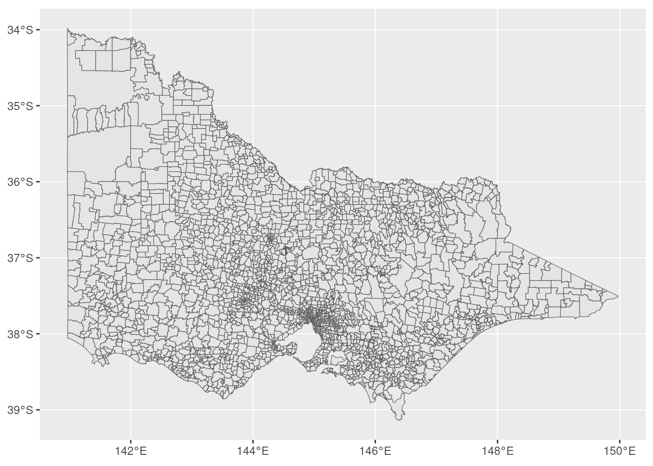
These borders are local government areas for the entire state of Victoria, Australia. The borders of these localities aren’t going to be exactly the same now as they were when the censuses were performed, but it’ll be good enough for our purposes. We’re only interested in the inner-Melbourne area, so we crop this to the relevant latitudes and longitudes:
inner_melb_localities <-
    vic_localities %>%
    st_crop(xmin=144.7, xmax=145.1, ymin=-37.95, ymax=-37.6)
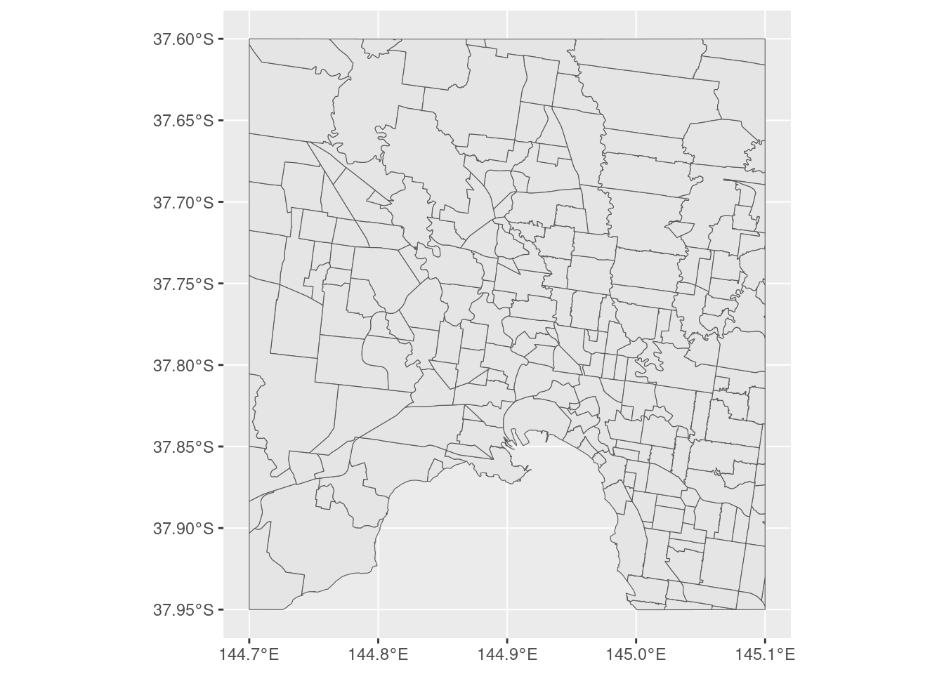
With our two key pieces of data in place, we can start to put them together.
Step 2 - Data Wrangling
Next step is to merge our migration data with our geospatial data using the suburb as our key, however it’s a little more complex that a simple join. As we want to ensure for every year we have all of the geospatial information so as to render the full map, we need to do a bit of group()ing and nest()ing.
The way I’ve tackled this is as such:
- Group by each year.
- Nest the data based on these groups.
- Perform a join on this nested data with the spatial data.
- This way we ensure that for each year, the spatial data for each suburb is present and the map is complete.
- Unnest the data
- For suburbs that don’t have any data for a particular census, we assign them 0 in the Percetnage and Total columns.
- I talked to Jen about this, and she made a decision in the short term to replace these with 0.
- Were more rigor required for the visualisation, other options would need to be considered to better portray this missing data.
- Convert to a geospatial object.
Below is the full pipeline, interspersed with comments to help understand what’s happening in each stage:
migrant_data_geo <-
    migrant_data %>%
    group_by(Year) %>%
    nest() |>
    # On a per census year basis, join each year's data with the spatial data
    mutate(
        geo = map(data, ~{ right_join(.x, inner_melb_localities, by = c('Suburb' = 'LOC_NAME')) })
    ) %>%
    unnest(geo) |>
    arrange(Suburb) %>%
    # Replace the NAs due to missing data with zero
    mutate(
        Percentage = replace_na(Percentage, 0),
        Total = replace_na(Total, 0),
    ) %>%
    select(-data) %>%
    ungroup() %>%
    # Convert back to a 'simple features' (geosptatial) object
    st_as_sf()
Step 3 - Rendering
The final step is the easiest: the rendering. The map is rendered with the fill of each polygon representing the percentage of population born overseas. This is then animated, with the fill transitioning smoothly between each Year
migrant_data_geo_animation <-
    migrant_data_geo %>%
    ggplot() +
    geom_sf(aes(fill = Percentage)) +
    labs(
        title = "Melbourne - Percentage Residents Born Overseas",
        subtitle = "Census Year: {closest_state}"
    ) +
    theme(
        plot.title = element_text(size = 10),
        plot.subtitle = element_text(size = 8),
        legend.title = element_text(size = 8),
        legend.text= element_text(size = 6)
    ) +
    scale_fill_distiller(name = "Percent", trans = 'reverse', labels = percent) +
    transition_states(Year, transition_length = 3, state_length = 5)
What we have in the end is what I handed over to Jen for her presentation: an animation showing the change in overseas-born population in inner-city Melbourne from 1954 to 1971.
Is That It?
Is this visualisation perfect? Far from it. There’s probably two areas where it could be improved. The first (and least important) is the aesthetics of it; I think it could simply look better. Better fonts, better arrangement, different colours.
But more importantly I think there that there are choices to be made about how the information is presented. The suburbs with no information have been zeroed out, is that the right choice? Does the colour scale accurately convey the change, or does it need to have multiple colours in it? Do the suburbs need to be labelled? What exactly is the definition of “inner-north Melbourne”?
All of those are decisions best made by someone with domain-specific knowledge, not necessarily by the person who’s generating the visualisation. Regardless, if we’re looking at this through an 80/20 lens, I contiue to be amazed about the 80 that can be generated with only a few lines of R code.