Simulating Snakes and Ladders
For the past couple of months my family and I - like the rest of the world - have been in isolation due to the coronavirus. My eldest son Ned is 5 years old and is interested in games and puzzles at moment, so these have been a key tool in reducing the boredom of lockdown.
Snakes and ladders is one of the games that’s caught his attenton. While sitting on the floor and playing a game for the umpteenth time, I started to wonder about some of the game’s statistical properties. That’s normal, right?
In this article I want to try and answer two questions about snakes and ladders. The first is:
For my son’s board, what is the average amount of dice rolls it takes to finish a game?
And the second is:
What is the average amount of dice rolls it takes to finish a game for a generalised board?
Defining the Board
This is the board we play on - it’s large sheet of plastic, hence the crinkles:
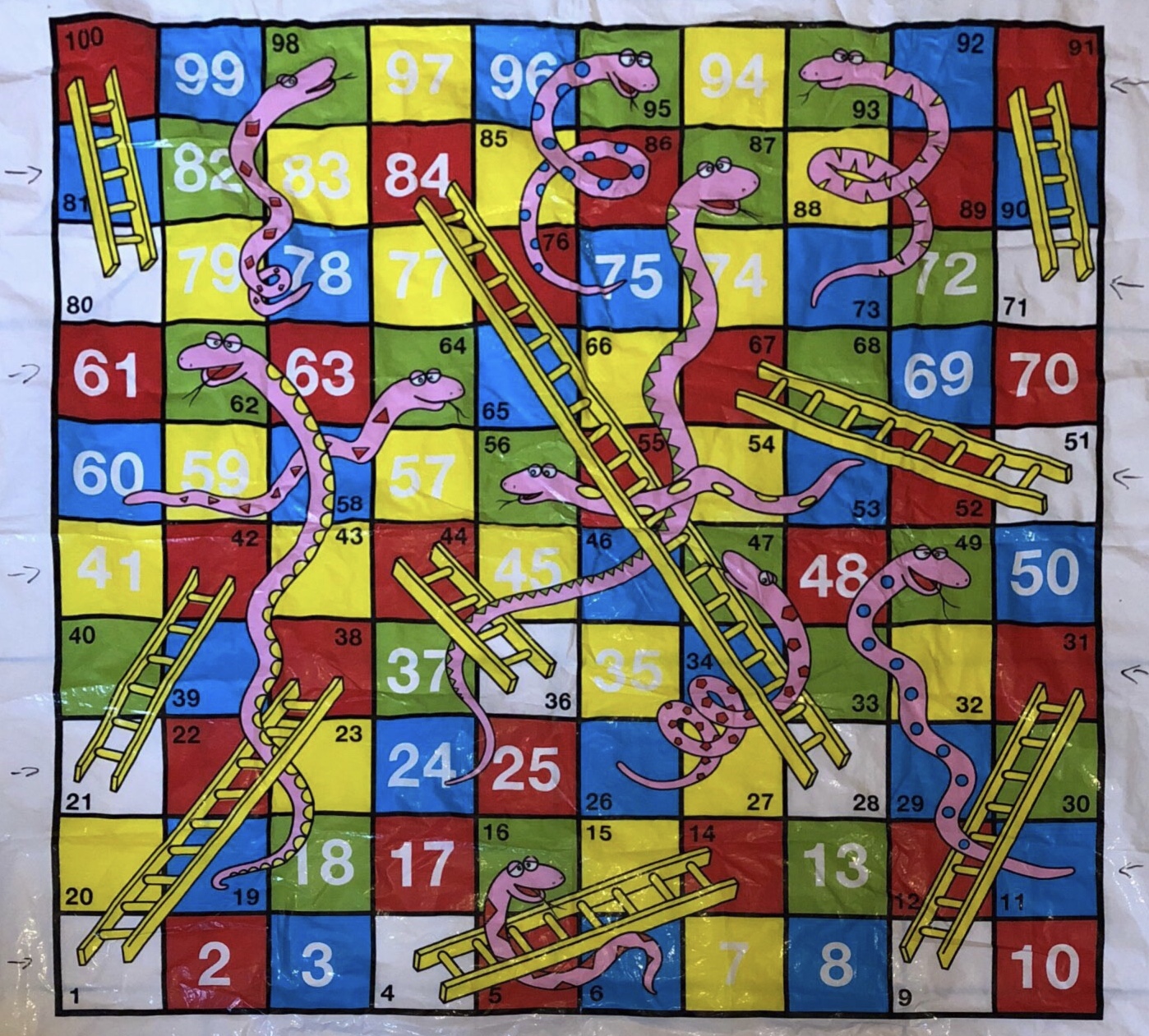
A snakes and ladders board can be represented as a vector, with each element of the vector representing a square or ‘spot’ on the board. Each element holds the value of the shift that occurs when you land on it: negative for snakes, positive for ladders, or zero for neither.
The vector below is a representation of my son’s board. We’re letting R do the calculations for us here, entering values as destination - source for ladders and source - destinaton for snakes.
neds_board = c(
    38-1, 0, 0, 14-4, 0, 0, 0, 0, 31-9, 0,
    0, 0, 0, 0, 0, 6-16, 0, 0, 0, 0,
    42-21, 0, 0, 0, 0, 0, 0, 84-28, 0, 0,
    0, 0, 0, 0, 0, 44-36, 0, 0, 0, 0,
    0, 0, 0, 0, 0, 0, 26-47, 0, 11-49, 0,
    67-51, 0, 0, 0, 0, 53-56, 0, 0, 0, 0,
    0, 19-62, 0, 60-64, 0, 0, 0, 0, 0, 0,
    91-71, 0, 0, 0, 0, 0, 0, 0, 0, 100-80,
    0, 0, 0, 0, 0, 0, 24-87, 0, 0, 0,
    0, 0, 73-93, 0, 75-95, 0, 0, 78-98, 0, 0
)
Playing the Game
With a data structure that represents the board, we now we need an algorithm that represents the game.
The snl_game() function takes a vector defining a board, and a finish type, and runs through a single player game until the game is complete, returning the number of rolls it took to finish the game.
The finish type specfies one of the two different ways a game can be finished. My son and I play an ‘over’ finish type, where any dice roll that takes you over the last spot on the board length results in a win.
The other finish is the ‘exact’ type, where you need to land exactly one spot past the last spot on the board to win. If you roll a value that takes you over, you remain in your current place.
library(tidyverse)
library(magrittr)
library(glue)
library(knitr)
library(kableExtra)
snl_game <- function(board, finish = 'exact') {
    if (!finish %in% c('exact', 'over')) {
        stop("Argument 'finish' must be either 'exact' or 'over")
    }
    # We sart on 0, which is off the board. First space is 1
    pos <- 0
    # We finish one past the end of the board
    fin_pos <- length(board) + 1
    # roll counter
    rolls <- 0

    while (rolls <- rolls + 1) {
        # Roll the dice
        roll <- sample(1:6, 1)
        # Update the position
        next_pos <- pos + roll

        # Two types of finish:
        # a) We need an exact roll to win
        # b) We need any roll to win
        if (next_pos > fin_pos) {
            if (finish == 'exact')  { next }
            else                    { return(rolls) }
        }

        # Did we win?
        if (next_pos == fin_pos) { return(rolls) }

        # Take into account any snakes/ladders
        pos <- next_pos + board[next_pos]

        # Did we somehow move off the board in the negative direction?
        if (next_pos < 1) {
            warning(glue("Went into negative board position: {next_pos}"))
            return(NA_integer_)
        }
    }
}
Answering the Specific Question
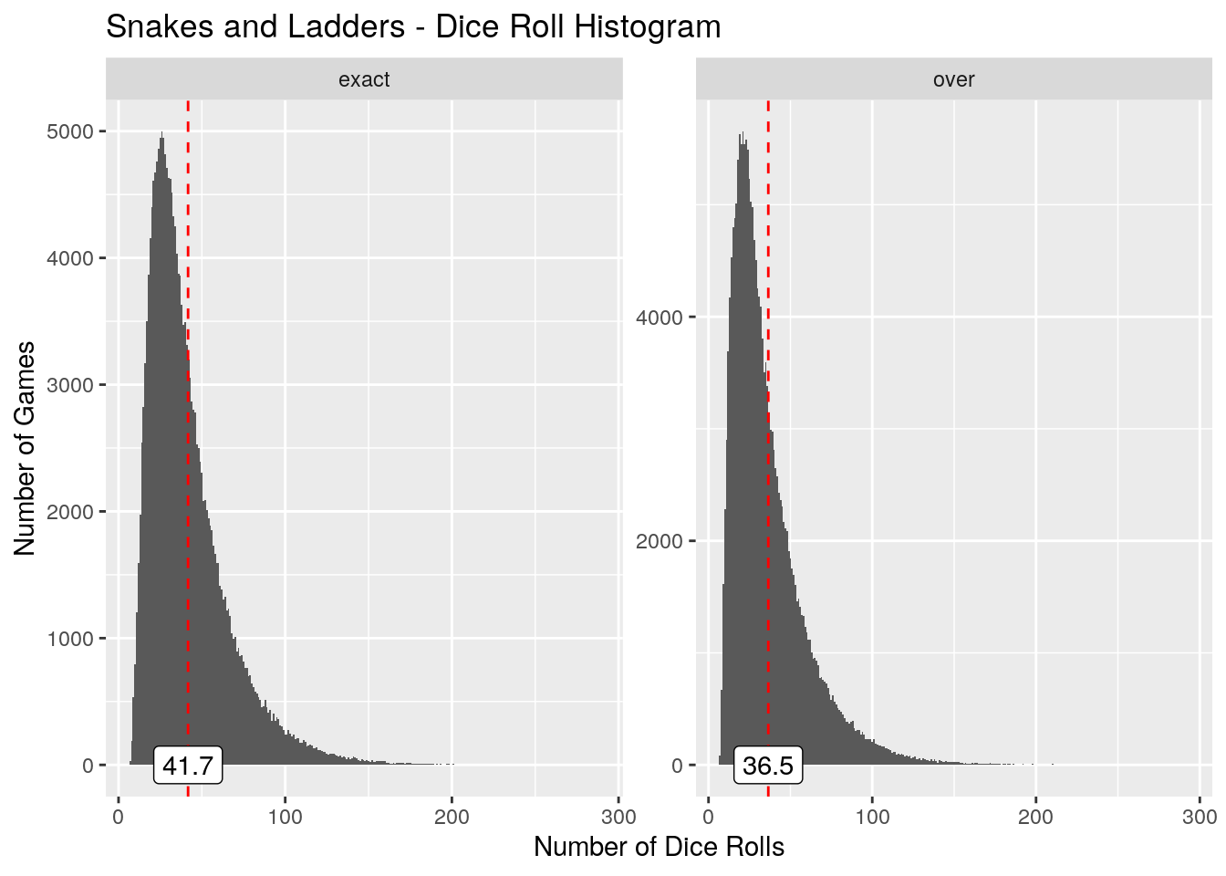
Now that we’ve defined a data structure and an algorithm, let’s try and determine the average number of rolls to win on my son’s board. Using my new favourite function crossing(), 200,000 games are simulated for each of the finish types and summary statistics calculated. We visualise the distribution of the numbner of rolls as a histogram:
# Simulate 200,000 games of each finish type
neds_board_sim <-
    crossing(
        finish_type = c('exact', 'over'),
        n = 1:200000
    ) %>%
    mutate(rolls = map_dbl(finish_type, ~snl_game(neds_board, finish = .x)))

# Summarise the results
neds_board_summary <-
    neds_board_sim %>%
    group_by(finish_type) %>%
    summarise(
        min = min(rolls),
        max = max(rolls),
        mean = mean(rolls),
        quantile_95 = quantile(rolls, .95),
        quantile_5 = quantile(rolls, .05)
    )

# Plot the histograms
neds_board_sim %>%
    ggplot() +
    geom_histogram(aes(rolls), binwidth = 1) +
    geom_vline(
        aes(xintercept = mean),
        linetype = 'dashed',
        colour = 'red',
        neds_board_summary
    ) +
    geom_label(aes(label = round(mean, 1), x = mean, y = 0), neds_board_summary) +
    facet_wrap(~finish_type, scales = 'free') +
    labs(
        x = 'Number of Dice Rolls',
        y = 'Number of Games',
        title = 'Snakes and Ladders - Dice Roll Histogram'
    )
print(neds_board_summary)
# A tibble: 2 x 6
  finish_type   min   max  mean quantile_95 quantile_5
  <chr>       <dbl> <dbl> <dbl>       <dbl>      <dbl>
1 exact           7   288  41.7          90         15
2 over            7   293  36.5          83         12
From this simulated data we’ve determined that it takes on average 41.72 rolls to finish an ‘exact’ game type, and 36.51 rolls to finish an ‘over’ game type.
For the ‘over’ finish type that my son and I play, I estimate a dice roll and move to take around 10 seconds. Our games should on average take around 13 minutes, with 95% of games finishing in less than 28 minutes.
Answering the General Question
We’ve answered the specific question, but can we generalise this to any board? To do this, we’ll have to provide a way of generating a board.
There are two random elements that we need to generate: which spots on the board will have a snake or a ladder, and the shift value for each of these spots.
The first step is to define the the shift - either forwards or backwards - of a single spot. This is done with the spot_alloc() function below. The shift is taken from a normal distribution (floored to an integer) and min()/max() clamped so that we don’t shift ourselves off the bottom or the top of the board.
spot_alloc <- function(spot, board_size, mean, sd) {
    # Integer portion of a random normal variable
    r <- floor(rnorm(1, mean, sd))

    # Clamp the shift value to within the board limits
    max(-(spot -1), min(board_size - spot, r))
}
The second step is to generate the board. The snl_board() function does this, taking a board size, a proportion of the board that will be snakes and ladders, and a desired mean and standard deviation for the snake and ladder shifts.
snl_board <- function(board_size, proportion, mean, sd) {
    # Allocate the board
    board <- rep(0, board_size)

    # Which spots will on the board will be snakes or ladders?
    spots <- trunc(runif(proportion * board_size, 1, board_size))

    # Assign to these spots either a snake or a ladder
    board[spots] <- map_dbl(spots, ~spot_alloc(.x, board_size, mean, sd))

    return(board)
}
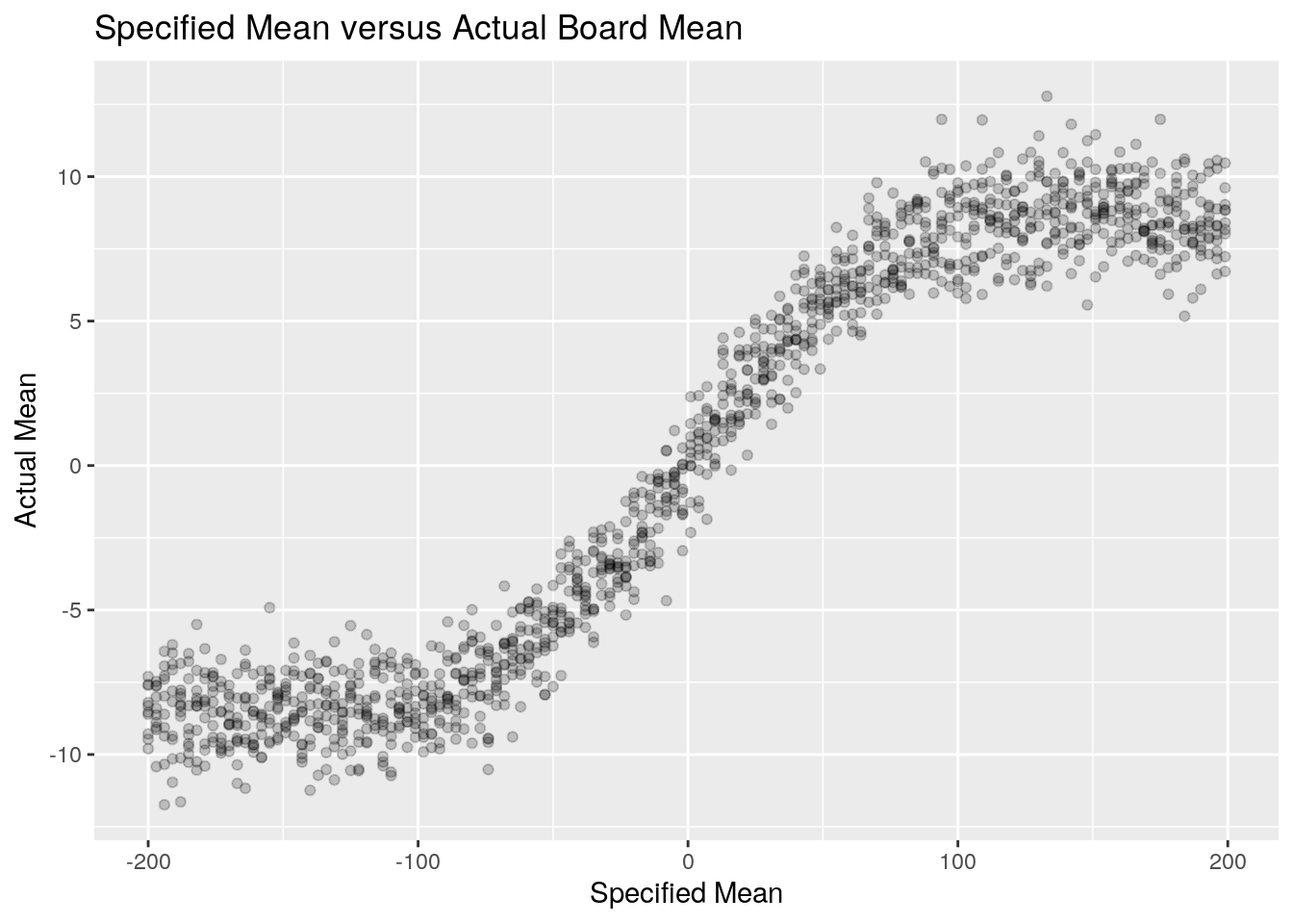
Due to the clamping, the mean we speciify in our argument to snl_board() doesn’t have a purely linear relationship to the evential mean of the entire board. We can see below that it actually resembles a logistic function.
# Our board generation with only one variable.
board_generator <- function(mean) {
    # Constant arguments across off of the simulations
   board_length <- 100
   snl_prop <- .19
   snl_sd <- board_length / 3

   snl_board(board_length, snl_prop, mean, snl_sd)
}

# Running the simulations
crossing(n = 1:10, mean = seq(-200, 200, 3)) %>%
    mutate( board_mean = map_dbl(mean, ~mean(board_generator(.x))) ) %>%
    ggplot() +
    geom_point(aes(mean, board_mean), alpha = .2) +
    labs(
        x = 'Specified Mean',
        y = 'Actual Mean',
        title = 'Specified Mean versus Actual Board Mean'
    )
With a board and a game we can now run our simulations for the general case. For each game type and mean we’ll run 200 simulations.
set.seed(1)
# Simulate our snakes and ladders games for different means and finish types.
general_snl_sim <-
    crossing(
        n = 1:200,
        mean = -2:100,
        finish_type = c('exact', 'over')
    ) %>%
    mutate(
        board = map(mean, ~board_generator(.x)),
        board_mean = map_dbl(board, ~mean(.x)),
        rolls = map2_dbl(board, finish_type, ~snl_game(.x, .y))
    )


general_snl_sim %>%
    ggplot() +
    geom_point(aes(board_mean, rolls, colour = finish_type), alpha = .5) +
    facet_wrap(~finish_type) +
    theme(legend.position = 'none') +
    labs(
        x = 'Board Mean',
        y = 'Number of Dice Rolls',
        title = 'Simulated Snakes and Ladders',
        subtitle = 'Mean of the Board vs. Number of Dice Rolls'
    )
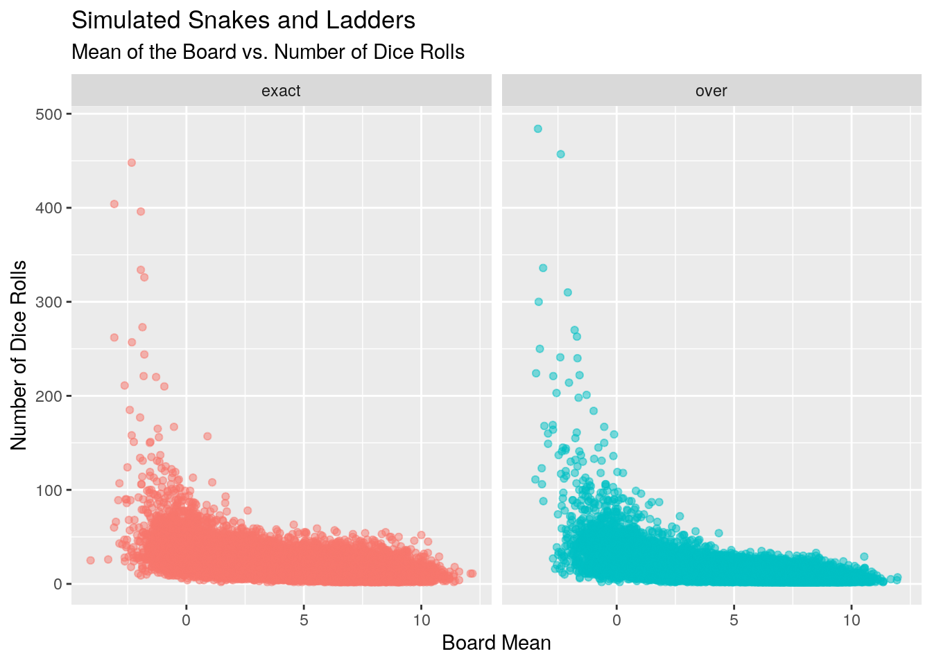
With the data in hand, we can now attempt to model the number of dice rolls versus the board mean to answer our question.
Modeling
We’ll keep it simple and apply an ordinary least squares to each of the finish types separately.
library(broom)

# Perform a regression against each group separately
ols_models <-
general_snl_sim %>%
    group_by(finish_type) %>%
    do(model = lm(rolls ~ board_mean, data = .) )

# Graph the linear regression
general_snl_sim %>%
    ggplot() +
    geom_point(aes(board_mean, rolls, colour = finish_type), alpha = .3) +
    geom_smooth(aes(board_mean, rolls), method = 'lm', formula = 'y ~ x', ) +
    facet_wrap(~finish_type) +
    labs(
        x = 'Board Mean',
        y = 'Dice Rolls',
        colour = 'Finish Type',
        title = 'Number of Dice Rolls vs Board Mean',
        subtitle = 'Split by Finish Type with OLS Best Fit'
    )
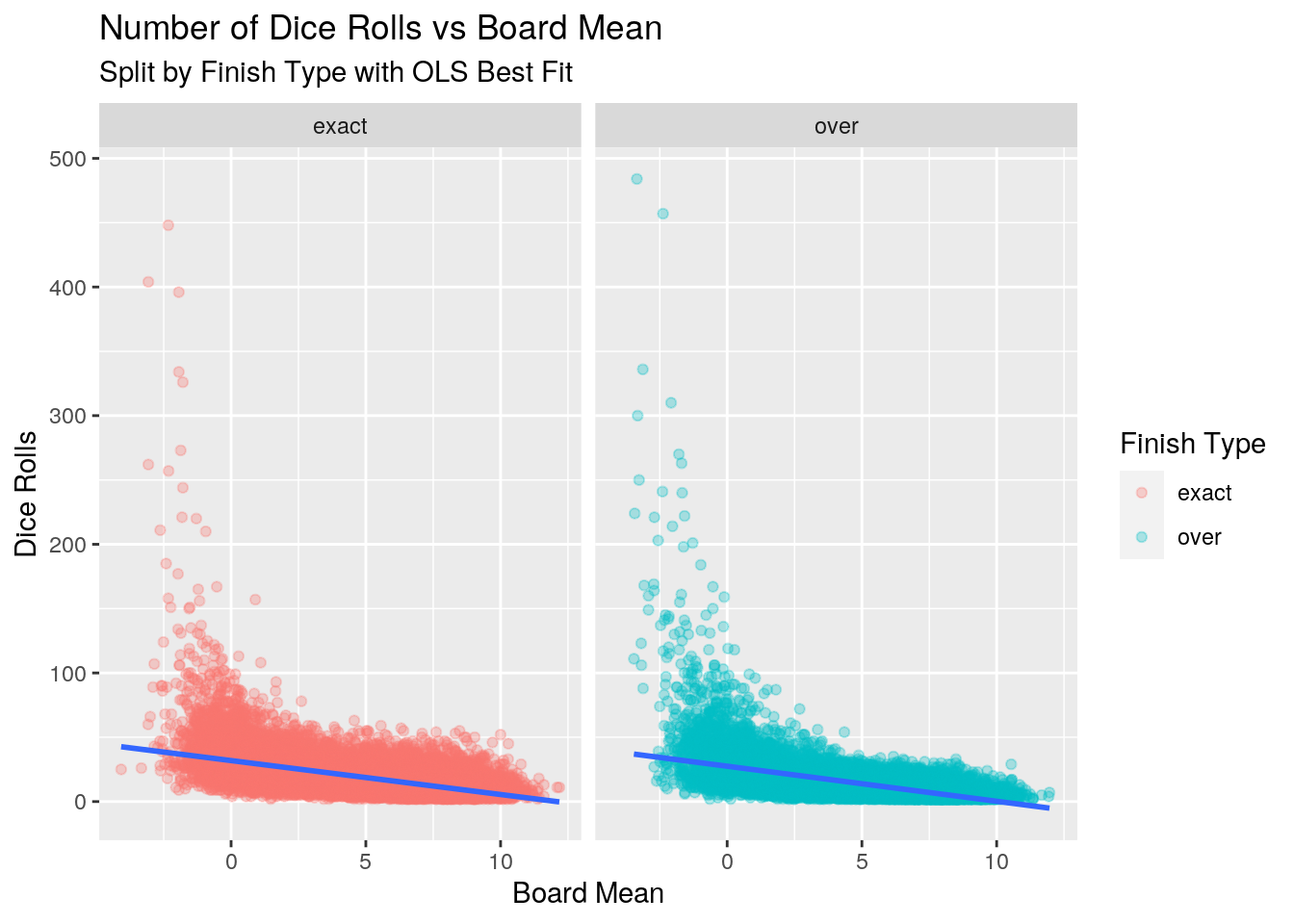
The intercepts, which represent a board mean of 0, are 31.9 rolls for the exact finish type, and 27.5 rolls for the over finish type.
The coefficient of the board mean variable is very similar for both finish types, -2.6 and -2.7 for the exact and over types respectively. This tells us that for every one unit increase in the board mean, the number of rolls to finish a game on average decreases by -2.6 and -2.7 rolls.
Whenever we discuss a linear model it’s not enough to simply discuss coefficients; we also need to discuss what our uncertaintly is. However let me put a pin in this and discuss this shortly when looking at the diagnostics of the fit.
ols_models %>% tidy(model)
# A tibble: 4 x 6
# Groups:   finish_type [2]
  finish_type term        estimate std.error statistic p.value
  <chr>       <chr>          <dbl>     <dbl>     <dbl>   <dbl>
1 exact       (Intercept)    31.9     0.181      176.        0
2 exact       board_mean     -2.64    0.0318     -82.9       0
3 over        (Intercept)    27.5     0.172      160.        0
4 over        board_mean     -2.72    0.0302     -90.1       0
How well does the least squares model the number of roles in terms of the mean of the board? The R-squared value tells us that the linear regression explains around 25% for the exact finish type, and 28% for the over finish type. On first glance that seems low, however it’s probably reasonable given the randomness of the dice rolls and the snakes and ladders.
ols_models %>%
    glance(model) %>%
    select(finish_type, r.squared)
# A tibble: 2 x 2
# Groups:   finish_type [2]
  finish_type r.squared
  <chr>           <dbl>
1 exact           0.250
2 over            0.283
The next step is to perform some diagnostics on these models. The first thing to look at is a graph of the residuals versus the response variable.
ols_models %>%
    augment(model) %>%
    ggplot() +
    geom_point(aes(.fitted, .resid, colour = finish_type), alpha = .1) +
    geom_smooth(aes(.fitted, .resid), method = 'loess', formula = 'y ~ x') +
    facet_wrap(~finish_type) +
    labs(
        x = 'Fitted Value',
        y = 'Residuals',
        colour = 'Finish Type',
        title = 'Residual Diagnostic Plot'
    )
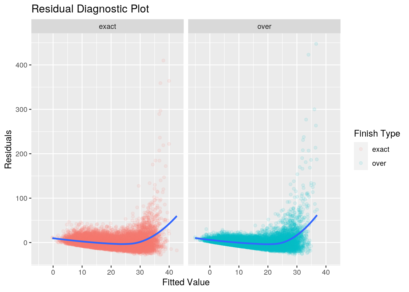
There are two things that immediately stand out in this plot - potential non-linearity of the data, the heteroscedacticity of the residuals.
Non-Linearity
Thie first property of the residual graph to notice is the uptick in the shape of the residuals between a fitted value of 30 and 40. This tells us that for fitted values less than 30 (or high board means), the linear regression is a resonably fit to the data. However as the fitted values grow, there doesn’t appear to be a linear relationship between the response and predictor.
The next steps from here would be to either transform the predictor before applying the linear regression, or finding a more flexible model to fit the data on.
Heterocedasticity
The second property to notice is the variance of the residuals increasing as the fitted values increase. This manifests itself as a funnel shape in the residual plot. Our residuals are heteroscedastic, rather than homoscedastic. An important assumption of a linear regression model is that the residuals have a constant variance. The standard errors and confidence intervals rely on this assumption.
This variability is the reason that we didn’t take a look at the standard error after performing our regression: given the variability of the residuals, the standard error is not liklely to be providing us with accurate information.
A possible solution to this is to transform the response using a consave function (square root or log). This results in a greater shrinkage for larger responses, leading to a redicution in heteroscedacticity.
Conclusion
At the ouset of this article I wanted to answer two questions: what is the mean number of rolls it takes to finish a snakes and ladders game on a specific board, and what is the mean number of rolls to finish a game on a general board.
In the specific instance we simulated a large number of games on the specific board. Using this data we were able to determine the mean rolls, as well and lower 5% and upper 95% bounds.
In the general instance we again simulated a large number of games on boards with different means. We it an ordinary least squares model to the data, but saw two issues: some non-linearity of the data in certain ranges of the independent variable, and heteroscedacticity of the residuals. Further work would be needed - either by transforming the data or by using a more flexible model - to get more accurate estimates and confidence intervals of the mean number of rolls across all board means.