A Brief Tour of Lebesgue Curves
Before we start a note: this post is a sidebar for another article I’m currently writing. There aren’t any grand conclusions or deep insights, it’s more exploratory.
Whilst writing an article on memory allocations, I needed a way to map a one-dimensional number (the memory location) on to two-dimensional space. By doing this I could visualise where in memory these allocation were occurring.
My initial reaction was to reach for the space-filling Hilbert curve à la the XKCD “Map of the Internet”, but whist researching I discovered the Lebesgue Curve, also known as the Z-order or Morton curve. At first glance it looked to have reasonable locality, and its inherent binary nature meant it appeared easier to implement.
In this article I’ll implement the Lebesgue curve and explore some of its properties.
Lebesgue Curve
The Lebesgue curve maps an one-dimensional integer into integers in two or more dimensions. In can also be used in reverse to map two or more integers back into a single integer. If we get a bit fancy with our notation, we can define the Lebesgue function \(l\) as:
$$ l : \mathbb{N} \to \mathbb{N^2} $$
where \(\mathbb{N}\) is the set of natural numbers, including 0.
The algorithm is relatively simple:
- Take an \(n\) bit integer \(Z\)
- Mask the even bits \([0, 2, \ldots, n - 2]\) into \(x\)
- Mask the odd bits \([1, 2, \ldots, n - 1]\) into \(y\)
- Collapse/shift the masked bits down so that they are “next” to each other
- This results in an \(\frac{n}{2}\) bit integer
In the C++ code below I’ve defined the lebesgue_coords() function that implements the above algorithm. It’s certainly not the most optimal implementation (it iterates through all the bits even if they’re 0), but it should have clarity. I’ve then vectorised it in the lebesgue() function that returns a list of \(x\) and \(y\) coordinates for each \(z\) integer, and exported using Rcpp so it can be used in the R environment:
#include <Rcpp.h>
using namespace Rcpp;

//The x,y vertice generated from the single z value
struct vert { unsigned long x; unsigned long y; };

//Lebesgue calculation for a single z value
struct vert lebesgue_coords(unsigned long z) {
    struct vert coords;
    unsigned long shift_mask;

    //Mask out even bits
    coords.x = z & 0x55555555;
    //Mask out odd bits, then shift back
    coords.y = (z & 0xaaaaaaaa) >> 1;

    //This bit compresses the masked out bits.
    //i.e. 1010101 -> 1111
    shift_mask = 0xfffffffc;
    do {
        //Extract the top bits, then shift them down one
        long int x_upper = (coords.x & shift_mask) >> 1;
        long int y_upper = (coords.y & shift_mask) >> 1;

        //Clear out the top bits from x and re-introduce
        //the shift top bits, thereby compressing them together
        coords.x = x_upper | (coords.x & ~shift_mask) ;
        coords.y = y_upper | (coords.y & ~shift_mask);

    } while (shift_mask <<= 1);

    return coords;
}

// [[Rcpp::export]]
List lebesgue(IntegerVector z) {
    int i;
    struct vert v;
    IntegerVector x,y;

    for (i = 0; i < z.size(); i++) {
        v = lebesgue_coords(z[i]);
        x.push_back(v.x);
        y.push_back(v.y);
    }
    return List::create(Named("x") = x, Named("y") = y);
}
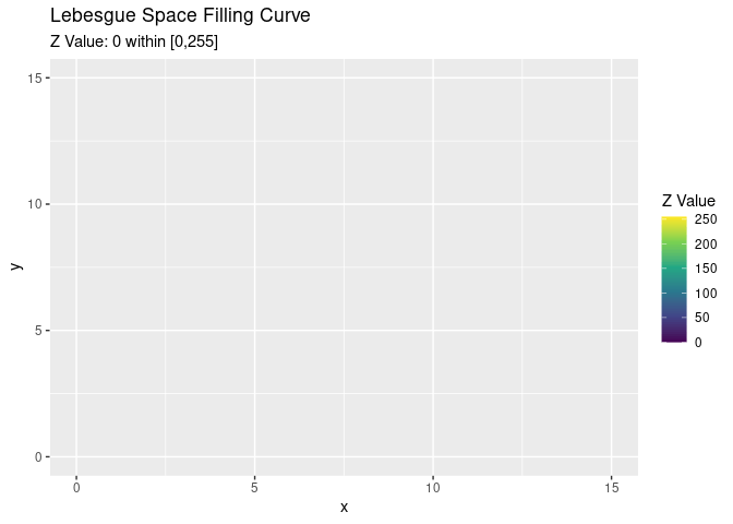
With this function we can have a look at how this function works across the integers \([0,255]\). You should be able to see the fractal-like behaviour, with clusters of 4, 16, 64, etc:
lebesgue_points <-
tibble(z = 0 : 255) |>
    mutate(l = as_tibble(lebesgue(z))) |>
    unnest(l)

print(lebesgue_points)
# A tibble: 256 × 3
       z     x     y
   <int> <int> <int>
 1     0     0     0
 2     1     1     0
 3     2     0     1
 4     3     1     1
 5     4     2     0
 6     5     3     0
 7     6     2     1
 8     7     3     1
 9     8     0     2
10     9     1     2
# … with 246 more rows
Locality
I mentioned at the start that the Lebesgue has ‘good locality’, but what exactly does this mean? There are multiple ways to define it, with a more rigorous take in this paper. I’ll be a little more little more hand-wavy and define it as “points that are close together in one-dimensions should be close together in two dimensions.”
We’ll look at consecutive numbers - which have a distance of 1 in one-dimension - and compare their distance in two dimensions. More formally, we’ll determine see how far away \((x_{z},y_{z})\) is away from \((x_{z-1}, y_{z-1})\) using good old fashioned Pythagoras to determine the distance:
$$ d = \sqrt{(x_2 - x_1)^2 + (y_2 - y_1)^2} $$ Let’s take a look at the average distance between the \(z\) values \([0,255]\):
lebesgue_locality <-
    lebesgue_points |>
    mutate(
        coord_distance = sqrt(
            (x - lag(x,1))^2 +
            (y - lag(y,1))^2
        )
    ) |>
    filter(!is.na(coord_distance))

lebesgue_locality |>
    summarise(mean_distance = mean(coord_distance))
# A tibble: 1 × 1
  mean_distance
          <dbl>
1          1.56
So on average, each point is 1.56 times further away in the two dimensional representation that in the one-dimensional representation. But as we all (should) know, an average is a summary and hides specifics. Taking a look at \(z\) versus the distance paints a more accurate picture of the underlying process:
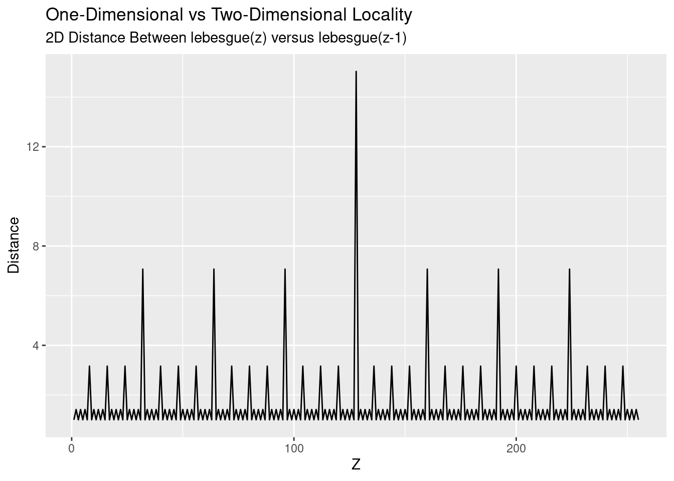 Locality is good, except every so often we get a spike of distance between points. This spike is where we’re moving between our different power-of-two regions: \(2^4, 2^6, 2^8, \ldots\). For a different perspective, we map our two-dimensional points with colour and size conveying the distance:
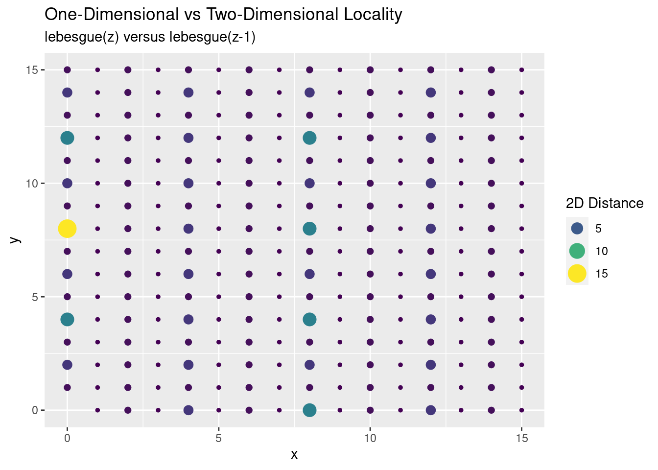
We see the large outlier, but in general most points are reasonably close to each other. More importantly it should be good enough for my original purposes.
Additive Properties
Finally, we’ll look at some additive properties that yielded an interesting result. As part of the aforementioned article I am using the Lebesgue curve in, a really useful property would have been this:
$$ l(a + b) = l(a) + l(b) $$ Unfortunately I quickly determined that this was not the case:
lebesgue(0:10 + 3)$x == lebesgue(0:10)$x + lebesgue(3)$x
[1] TRUE TRUE FALSE TRUE TRUE FALSE FALSE FALSE TRUE TRUE FALSE
As I played around with different ranges and different addends, I couldn’t discern the pattern. The next move was to visualise it to try and better understand the interaction.
We do this in the code below. The crossing() is a handy function to know, generating which generates all 128x128 combinations of the integers 0 through 127. For each of these pairs, we determine whether adding each combination inside the function versus individually leads to a true or false result. The result of this boolean is then visualised on each point on the graph:
equality <-
    crossing(a = 0:127, b = 0:127) |>
    mutate(
        x = (lebesgue(a + b))$x == (lebesgue(a)$x + lebesgue(b)$x),
        y = (lebesgue(a + b))$y == (lebesgue(a)$y + lebesgue(b)$y)
    ) |>
    pivot_longer(cols = c(x, y), names_to = 'coord', values_to = 'equality')

print(equality)
# A tibble: 32,768 × 4
       a     b coord equality
   <int> <int> <chr> <lgl>
 1     0     0 x     TRUE
 2     0     0 y     TRUE
 3     0     1 x     TRUE
 4     0     1 y     TRUE
 5     0     2 x     TRUE
 6     0     2 y     TRUE
 7     0     3 x     TRUE
 8     0     3 y     TRUE
 9     0     4 x     TRUE
10     0     4 y     TRUE
# … with 32,758 more rows
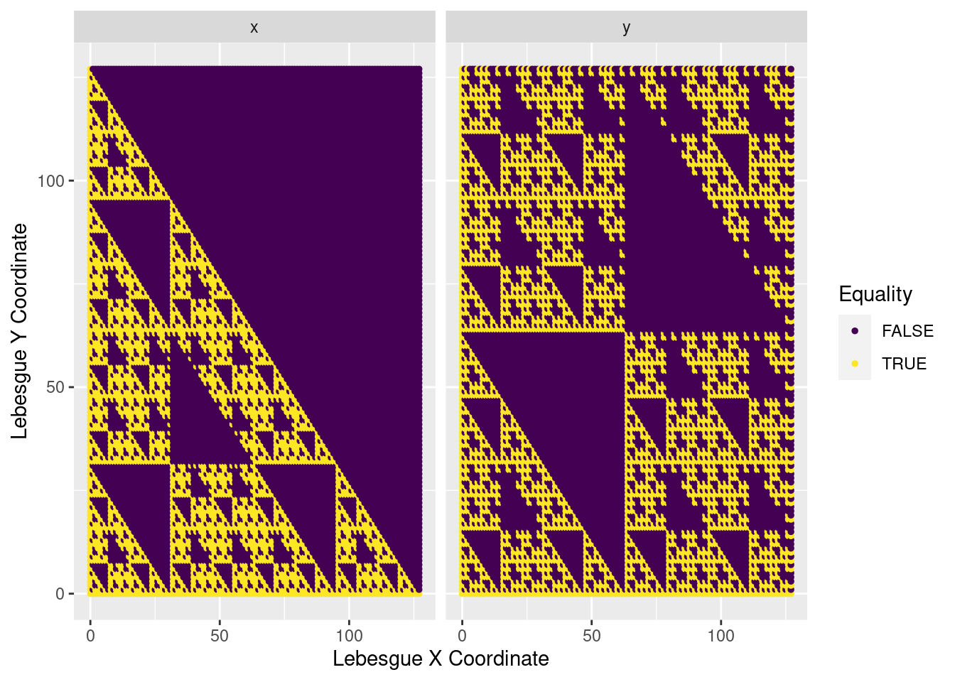 I must admit, I was a bit stunned when I saw this pop out; it was not at all what I expected. You can see some interesting fractal behaviour, with each boolean pattern being repeated in larger and larger sections. It looks a little like a Sierpiński triangle, but I’m not sure if there’s any relation. It may be somewhat anticlimactic, but I haven’t delved any deeper into this. That gets added to the ever-growing todo list.
Summary
In this article we had a brief, exploratory look at the space-filling “Lebesgue” curve. We looked at how it’s implemented, some of its locality behaviour, and some interesting results under addition. In a future article we’ll use this algorithm to help visualise the dynamic memory allocations of a process.