AFL Bets - Analysing the Halftime Payout
If you’ve watched AFL over the past few years, you would have noticed betting companies spruiking a cornucopia of betting options. In fact it would be hard for you not to notice, given the way they yell at you down the television screen.
One of the value adds these companies advertise is the ‘goal up at halftime’ payout. The terms are that if you have a head-to-head bet on the game, and your team is up by 6 points or more at half time, you’ll be paid out as if you had won.
Betting companies aren’t in the business of giving away money, so they must be confident that, in the long run, the team that is up at half time almost always goes on to win the game. But how confident should they be? Is this something that we can calculate?
Good data analysis always starts off with a question. In this article I will try to answer the question:
If a betting company pays out an AFL head-to-head bet at halftime because a team is up by 6 points or more, in the long run what proportion of bets will the betting company payout that they wouldn’t have if they didn’t offer this option?
There are two scenarios to consider:
- A team is up at half time and goes on to win.
- A team is down at half time and goes on to win.
With 1, a betting company loses nothing paying out at half time, as they will have had to have paid out the bet anyway. However with 2, the betting company does lose, as they’re paying out both teams. We want to determine how often this scenario plays out.
Model Notes Assumptions
The terms of the payout are clear-cut: head-to-head bet, team is up by a goal, bet is paid out. We want to model the probability of a win (the result) versus the half time differential (the predictor):
$$ Pr(R = Win | S) $$
Where \(R\) is the result (Win, Loss), and \(S\) is the score differential at halftime.
The main assumption we need to make is around timing: we assume that this halftime payout is applied across all games. This allows us to discount all other variables such as the teams’ odds, weather conditions, team form, etc. What is likely is that the betting companies have far more complex statistical models that take into account a wide range of variables. They can then ‘turn on’ this offer on specific games when the probabilities are in their favour.
Another item to consider is how far to go back in time to train our model. It could be that the game has changed significantly in the past few years, making this kind of payout more feasible. We will attempt to model this by adding a categorical variable representing the league a game was played in: the Victorian Football League (VFL) or the Australian Football League (AFL). We can then determine whether this has statistical significance, and whether it increases the accuracy of our model.
What About a Draw?
Spoiler alert: we’re going to be using a logistic regression in our model. This allows us to model a binary outcome, but we actually have three outcomes: loss, win and draw.
In a draw, the head-to-head bet is paid out at half the face value. So if a team is up at halftime and paid out, and the game goes on to be a draw, the betting company will still have paid out more than they had to. As we’re looking at ‘the proportion of bets the betting company payout that they wouldn’t have if they didn’t offer this option’, we will consider a draw to be a loss.
Loading and Transforming the Data
Our data for this analysis will come from the AFL Tables site, via the fitzRoy R package. The data is received in a long format that includes statistics for each player. We’re only concerned with team statistics, not player statistics, so the first row is taken from each game and transmuted into the variables we require.
As discussed in the assumptions, we’d like to see if there’s a difference between the VFL and AFL leagues. A categorical variable is added denoting whether the game was played as part of the ‘Australian Football League’ or ‘Victorian Football League’, which changed in 1990.
library(tidyverse)
library(magrittr)
library(fitzRoy)
library(modelr)
library(lubridate)

# Download the AFL statistics
afl_match_data <- get_afltables_stats()

# Group by each unique game and take the first row from each.
# Transmute into the required data.
afl_ht_results <-
    afl_match_data %>%
    mutate(
        Game_ID = group_indices(., Season, Round, Home.team, Away.team)
    ) %>%
    group_by(Game_ID) %>%
    slice(1) %>%
    transmute(
        Home_HT.Diff = (6 * HQ2G + HQ2B) - (6 * AQ2G + AQ2B),
        Away_HT.Diff = -Home_HT.Diff,
        Home_Result = as_factor(ifelse(Home.score > Away.score, 'Win', 'Loss')),
        Away_Result = as_factor(ifelse(Away.score > Home.score, 'Win', 'Loss')),
        League = ifelse(year(Date) >= 1990, 'AFL', 'VFL')
    ) %>%
    ungroup()

print(afl_ht_results)
# A tibble: 15,705 x 6
   Game_ID Home_HT.Diff Away_HT.Diff Home_Result Away_Result League
     <int>        <dbl>        <dbl> <fct>       <fct>       <chr>
 1       1           13          -13 Win         Loss        VFL
 2       2            2           -2 Win         Loss        VFL
 3       3          -18           18 Loss        Win         VFL
 4       4          -17           17 Loss        Win         VFL
 5       5          -14           14 Loss        Win         VFL
 6       6           20          -20 Win         Loss        VFL
 7       7           23          -23 Win         Loss        VFL
 8       8          -41           41 Loss        Win         VFL
 9       9          -24           24 Loss        Win         VFL
10      10          -15           15 Loss        Win         VFL
# … with 15,695 more rows
We have one row per game, but our observations are focused on each team rather than each individual game. We pivot the data to give us the half time differential and result per team, which results in two rows per game. Note the ability of pivot_longer() to extract out more than two columns at once using the names_sep argument.
afl_ht_results <-
    afl_ht_results %>%
    pivot_longer(
        -c(Game_ID, League),
        names_to = c('Team', '.value'),
        names_sep = '_',
        values_drop_na = TRUE
    ) %>%
    select(-Team)

print(afl_ht_results)
# A tibble: 31,410 x 4
   Game_ID League HT.Diff Result
     <int> <chr>    <dbl> <fct>
 1       1 VFL         13 Win
 2       1 VFL        -13 Loss
 3       2 VFL          2 Win
 4       2 VFL         -2 Loss
 5       3 VFL        -18 Loss
 6       3 VFL         18 Win
 7       4 VFL        -17 Loss
 8       4 VFL         17 Win
 9       5 VFL        -14 Loss
10       5 VFL         14 Win
# … with 31,400 more rows
In this format there is a lot of redundancy: each game has two rows in our data frame, with each row simply being the negation of the other row. We remove this redundancy by taking, at random, either one team’s variable from each game.
At this point, we have tidied and transformed our data into the variables we require and into the shape we need. We can now start to analyse and use it for modeling.
afl_ht_sample <-
    afl_ht_results %>%
    group_by(Game_ID) %>%
    sample_frac(.5) %>%
    ungroup()

print(afl_ht_sample)
# A tibble: 15,705 x 4
   Game_ID League HT.Diff Result
     <int> <chr>    <dbl> <fct>
 1       1 VFL         13 Win
 2       2 VFL          2 Win
 3       3 VFL        -18 Loss
 4       4 VFL        -17 Loss
 5       5 VFL         14 Win
 6       6 VFL         20 Win
 7       7 VFL         23 Win
 8       8 VFL        -41 Loss
 9       9 VFL         24 Win
10      10 VFL         15 Win
# … with 15,695 more rows
Let’s take a look at the win/loss ratios for each halftime differential, splitting on whether which league the game was played.
# Graph the win/loss ratios by the halftime differential
afl_ht_sample %>%
    group_by(HT.Diff, League) %>%
    summarise(Ratio = mean(Result == 'Win'), .groups = 'keep') %>%
    ggplot() +
    geom_point(aes(HT.Diff, Ratio, colour = League)) +
    labs(
        x = 'Half Time Difference',
        y = 'Win/Loss Ratio',
        title = 'AFL Games - All Games',
        subtitle = 'Half Time Difference vs. Win/Loss Ratio'
    )
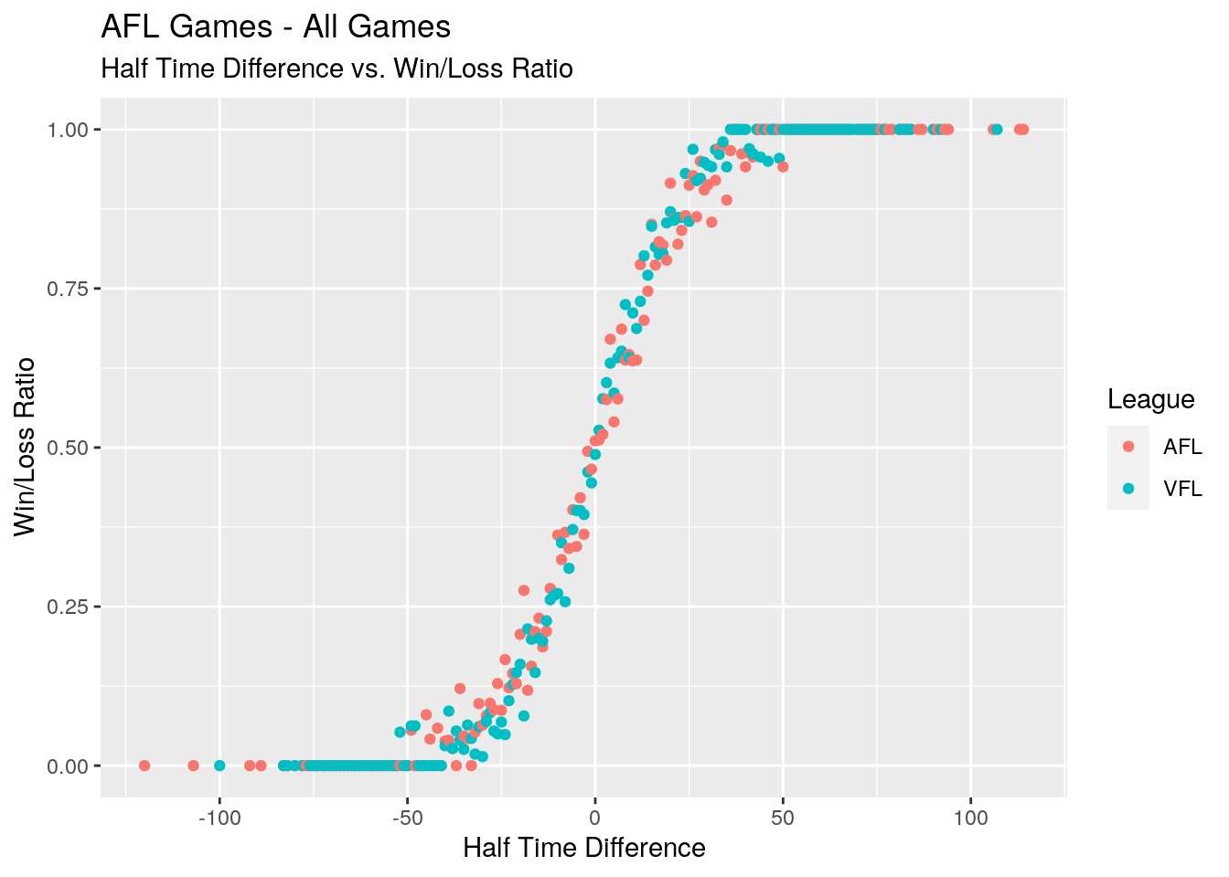
As mentioned earlier, we knew that the logistic regression would be the likley method used to model this data. This graph, with it’s clear sigmoid-shaped curve, confirms that a logistic regression is an appropriate choice.
Modeling
Our data is in the right shape, so we now use it to create a model. The data is split into training and test sets, with 80% of the observations in the training set and 20% left over for final testing.
A logistic regression is then used to model the result of the game against the halftime differential, the league, and also take into account any interaction between the league and the halftime differential. As a learning exercise I’ve decided to use the tidymodels approach to run the regression.
library(tidymodels)

# Split the data into training and test sets.
set.seed(1)
afl_ht_sets <-
    afl_ht_sample %>%
    initial_split(prop = .8)

# Define our model and engine.
afl_ht_model <-
    logistic_reg() %>%
    set_engine('glm')

# Fit our model on the training set
afl_ht_fit <-
    afl_ht_model %>%
    fit(Result ~ HT.Diff * League, data = training(afl_ht_sets))
Let’s see how this model looks against the the training data:
# View the logistic regression against the win/loss ratios
training(afl_ht_sets) %>%
    group_by(HT.Diff, League) %>%
    summarise(Ratio = mean(Result == 'Win'), .groups = 'keep') %>%
    bind_cols(predict(afl_ht_fit, new_data = ., type = 'prob')) %>%
    ggplot() +
    geom_point(aes(HT.Diff, Ratio, colour = League), alpha = .3) +
    geom_line(aes(HT.Diff, .pred_Win, colour = League))
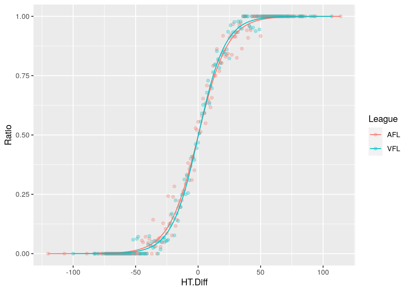
We see it fits the data well, and that there doesn’t appear visually to be much of a difference between the VFL era and the AFL era.
Probabilities
We’re concerned with half time differentials above 6, so let’s look at some of the probabilities our model spits out for one, two and three goal leads at half time.
# 1, 2 and 3 goal leads in the two leagues
prob_data <-
    crossing(
        HT.Diff = c(1, 2, 3) * 6,
        League = c('AFL', 'VFL')
    )

# Prediction across this data
afl_ht_fit %>%
    predict(new_data = prob_data, type = 'prob') %>%
    bind_cols(prob_data) %>%
    mutate(Percent_Win = round(.pred_Win * 100, 2)) %>%
    select_at(vars(-starts_with('.pred')))
# A tibble: 6 x 3
  HT.Diff League Percent_Win
    <dbl> <chr>        <dbl>
1       6 AFL           62.1
2       6 VFL           63.0
3      12 AFL           73.1
4      12 VFL           74.9
5      18 AFL           81.9
6      18 VFL           83.9
Our model gives mid-60%, mid-70% and mid-80% probabilities in both leagues for teams leading by one, two and three goals respectively. For the purposes of this article we’re going to use a decision threshold of 50% as between the ‘Win’ and ‘Loss’ categories.
What this means is that our model will always predict a win if a team is leading by a goal or more, and thus for the us there will only be two error types:
- True Positives - predicting a win when the result is a win.
- False Positives - predicting a win when the result is a loss.
At this point we could move to estimate the expected proportion of payouts simply looking at the win/loss ratios for halftime differentials of 6 point or more. But before we do that, let’s perform some further diagnostics on our model to ensure that we’re not making invalid assumptions.
Training Accuracy
The next step is to look at the accuracy of our model against the training set - that is - the same set of data that model was built upon.
# Calculate training accuracy
afl_ht_fit %>%
    predict(training(afl_ht_sets)) %>%
    bind_cols(training(afl_ht_sets)) %>%
    accuracy(Result, .pred_class)
# A tibble: 1 x 3
  .metric  .estimator .estimate
  <chr>    <chr>          <dbl>
1 accuracy binary         0.784
So 78.4% of the time the model predicts the correct result. That’s good, but we need to remember that the model was generated from the same data so it’s going to be optimistic. THe test accuracy is likely to be lower.
Model Coefficients
We’ve looked at the outputs of the model: probabilities and accuracy. But what is the model actually telling us about the relationship between halftime differential and league to the probability of a win? This is where the actual values of the model coefficients come in. Our logistic function will look as such:
$$ p(X) = \frac{ e^{\beta_0 + \beta_1 X_1 + \beta_2 X_2 + \beta_3 X_1 X_2} }{ 1 - e^{\beta_0 + \beta_1 X_1 + \beta_2 X_2 + \beta_3 X_1 X_2} }$$`
where \(X_1\) is the halftime differential in points, and \(X_2\) is a categorical variable denoting the league the game was played in: ‘AFL’ or ‘VFL’.
We also need to remember that the result of our model is not a probability, but the log-odds or logit of the result:
$$ logit(p) = log(\frac{p}{1 - p}) $$ where \(p\) is the probability of the result being a win.
# Model coefficients
afl_ht_fit %>%
    tidy()
# A tibble: 4 x 5
  term              estimate std.error statistic   p.value
  <chr>                <dbl>     <dbl>     <dbl>     <dbl>
1 (Intercept)        0.0139    0.0392      0.355 7.23e-  1
2 HT.Diff           -0.0846    0.00252   -33.6   8.02e-248
3 LeagueVFL          0.0126    0.0487      0.259 7.96e-  1
4 HT.Diff:LeagueVFL -0.00869   0.00332    -2.62  8.76e-  3
The model coefficients are as such:
- The intercept (\(\beta_0\)) tells us the log-odds of winning in the AFL with a halftime differential of zero.
HT.Diff(\(\beta_0\)) is the change in log-odds of a win in the AFL for every one point of halftime differential.LeagueVFL(\(\beta_1\)) tells us the difference in log-odds of winning with a differential of zero in the VFL as compared to the AFL.- This needs to be added to the intercept to when considering VFL games.
HT.Diff:LeagueVFL(\(\beta_3\)) is the difference in the change in log-odds of a win for every one point of halftime differential in the VFL.- Again, this needs to be added to the
HT.Diffvariable when considering VFL games.
- Again, this needs to be added to the
So for an AFL game, for each point a team is leading by at half time, their odds of winning increase by \(e^{-0.0846468}\) or 0.9188368. For a VFL game, it’s \(e^{-0.0846468 + (-0.0086936)}\) or 0.9108834.
Looking at the p-values, if we assume a standard significance value of \(\alpha = 0.05\), then the halftime difference is highly significant, and that there is a slight significance between the change in log-odds per halftime differential between the VFL and the AFL. So we can say that the odds of winning given a lead at halftime were slightly less in the VFL era as compared to the AFL era.
We’re building this model in order to predict the results, not in order to explain how each variable affects the outcome. As such, the statistical significance of each predictor isn’t that relevant to us. But it does raise a question: should we include the statistically insignificant predictors in our model or not?
To answer this question, we’ll use bootstrapping.
Bootstrapping
With the bootstrap, we take a sample from the training set a number of times with replacement, run our model across this data, and and record the accuracy. The mean accuracy is then calculated across all of these runs.
We’ll create two models: one with the league included, and a model without. The model with the best accuracy from this bootstrap is the model that will be used.
# Recipe A: Result vs Halftime Difference
afl_recipe_ht <-
    training(afl_ht_sets) %>%
    recipe(Result ~ HT.Diff) %>%
    step_dummy(all_nominal(), -all_outcomes())

# Bootstrap Recipe A
workflow() %>%
    add_model(afl_ht_model) %>%
    add_recipe(afl_recipe_ht) %>%
    fit_resamples(bootstraps(training(afl_ht_sets), times = 50)) %>%
    collect_metrics()
# A tibble: 2 x 5
  .metric  .estimator  mean     n  std_err
  <chr>    <chr>      <dbl> <int>    <dbl>
1 accuracy binary     0.784    50 0.000765
2 roc_auc  binary     0.869    50 0.000646
# Recipe B: Result vs Halftime Difference, League, and interaction term
afl_recipe_ht_league <-
    training(afl_ht_sets) %>%
    recipe(Result ~ HT.Diff + League) %>%
    step_dummy(all_nominal(), -all_outcomes()) %>%
    step_interact(~League_VFL:HT.Diff)

# Bootstrap recipe B
workflow() %>%
    add_model(afl_ht_model) %>%
    add_recipe(afl_recipe_ht_league) %>%
    fit_resamples(bootstraps(training(afl_ht_sets), times = 50)) %>%
    collect_metrics()
# A tibble: 2 x 5
  .metric  .estimator  mean     n  std_err
  <chr>    <chr>      <dbl> <int>    <dbl>
1 accuracy binary     0.784    50 0.000618
2 roc_auc  binary     0.869    50 0.000525
The result: there is hardly any difference between a model with only halftime difference, and a model that takes into account the league the game was played in.
Final Testing
A model needs to be chosen, and so the model with the league predictor is the one that will be used. How does the model stack up against the test set:
afl_ht_fit %>%
    predict(testing(afl_ht_sets)) %>%
    bind_cols(testing(afl_ht_sets)) %>%
    accuracy(Result, .pred_class)
# A tibble: 1 x 3
  .metric  .estimator .estimate
  <chr>    <chr>          <dbl>
1 accuracy binary         0.787
Our test accuracy is in fact slightly better than our training accuracy!
This accuracy is across the whole gamut of halftime differentials, but we’re only concerned with halftime differentials of 6 points or more:
# Filter out differentials of 6 points or more
afl_ht_testing_subset <-
    testing(afl_ht_sets) %>%
    filter(HT.Diff >= 6)

# Apply the model to this subset of data
afl_ht_testing_subset_fit <-
    afl_ht_fit %>%
    predict(afl_ht_testing_subset) %>%
    bind_cols(afl_ht_testing_subset)

# Test set, goal or more accuracy
afl_ht_testing_subset_fit %>%
    accuracy(Result, .pred_class)
# A tibble: 1 x 3
  .metric  .estimator .estimate
  <chr>    <chr>          <dbl>
1 accuracy binary         0.835
Our model, applied to the subset of the test data we’re concerned with, is 84% accurate.
Conclusion
How do these values we’ve calculated relate to the payouts a betting company has to deliver? If a head-to-bet has been placed on a team and that team is up by 6 points or more at half time, we estimate that 84% of the time they will go on to win. The betting company would have had to pay this out anyway, so scenario does not have an affect on the payout.
However with the ‘payout at halftime’ deal in place, there are times when a team is down by 6 points or more and at half-time and goes on to win. From our model and data, we see this occurring 16% of the time.
Therefore, with this deal in place, on head-to-head bets, we would expect the betting companies to pay-out 16/84 or 19.05% more times than they would if the deal was not in place. We note that this includes where a the result is a draw, and the company would only pay out half of the head-to-head bet.