A Tale Of Two Optimisations
A couple of months ago I wrote a toy program called whitespacer. Ever since, I’ve had this gnawing feeling that I could have done it better; that it could have been written in a more performant manner. In this article I’ll take you through a couple of different ideas I came up with. We’ll profile and visualise their different performances and stumble upon some surprising behaviour. We’ll use this as an excuse to take a deeper dive into their behaviour at the CPU level and gain a better understanding about the perf performance analysis tool and branch prediction.
A Quick Recap
In a previous article I took you through the whitespacer program. Here’s a quick recap of what it does:
- Reads from standard in and writes to standard out.
- Works in an ‘encoding’ and ‘decoding’ mode’.
- In encoding mode it takes each of the four dibits (2 bits) of each byte and turns it into one of four whitespace characters (tab, new line, carriage return and space).
- Decoding mode does the reverse, taking groups of four whitespace characters and reconstituting the original byte.
Here’s the encoding function:
//Dibit to whitesapce lookup table (global variable)
char encode_lookup_tbl[] = { '\t', '\n', '\r', ' ' };

//Given a dibit, returns the whitespace encoding
unsigned char lookup_encode(const unsigned char dibit) {
    return encode_lookup_tbl[ dibit ];
}
I’ve omitted the decoding function for brevity, but it’s the same with a different lookup table.
Attempt 1: A Mathematical Function
What bothered me about the original implementation was the lookup table. Even though I knew they’d be cached, I still thought the memory accesses might have a detrimental affect on performance.
I had an idea about using mathematical functions (rather than the lookup table) to perform the encoding/decoding. This would remove the memory accesses and perhaps improve performance.
From somewhere I recalled that if we have a set of \(k + 1\) data points \((x_0, y_0),…, (x_k, y_k)\) where no two \(x_i\) are the same, we can fit a curve using a linear regression with a polynomial of degree \(k\). Here’s our table of data points:
# A tibble: 4 × 2
  dibit ascii_dec
  <int>     <int>
1     0         9
2     1        10
3     2        13
4     3        32
This means we can find \(\beta\) coefficients for the function
$$ f(x) = \beta_0 + \beta_1 x + \beta_2 x^2 + \beta_3 x^3 $$
such that when passed a dibit value it returns the appropriate whitespace character. We can also find the inverse polynomial \(f^{-1}(x)\) which takes a whitespace character and returns a dibit to be our decoding function. Let’s create linear regression models in R where whitespace is the table holding our dibit and whitespace values:
encode_model <-
    whitespace %>%
    lm(ascii_dec ~ dibit + I(dibit^2) + I(dibit^3), data = .)

decode_model <-
    whitespace %>%
    lm(dibit ~ ascii_dec + I(ascii_dec^2) + I(ascii_dec^3), data = .)
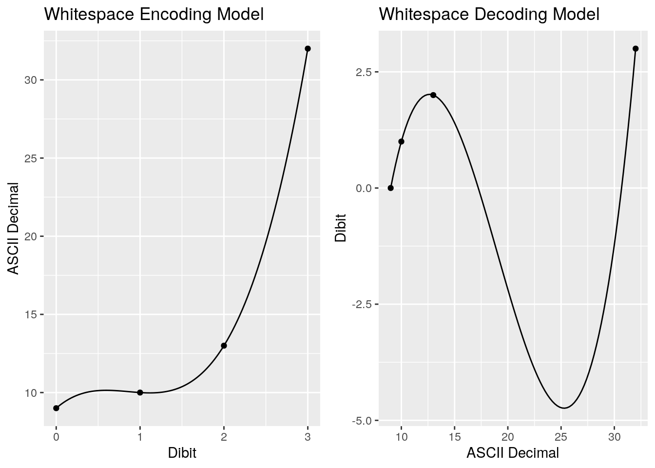
Visualising these models will help us see what’s going on. On the left is our encoding model, which takes out dibit values and maps them to our ASCII whitespace characters. On the right our decoding model, which takes the ASCII whitespace characters’ decimal value and maps it back to a dibit. What becomes obvious by visualising these is how they make no sense for any values outside of our four points:
Let’s take a look at the \(\beta\) coefficients:
# A tibble: 4 × 3
  parameter encode    decode
  <chr>      <dbl>     <dbl>
1 beta_0      9.00 -31.8
2 beta_1      4.67   6.42
3 beta_2     -6.00  -0.381
4 beta_3      2.33   0.00669
Immediately we see a bit of a problem. I’ll be honest that I was hoping - somewhat optimistically - for some nice, clean integer coefficients. Instead we’ve got floating point values. My gut feel is that having to use floating point instructions is not going to improve upon our original lookup table. But we won’t know until we profile, so let’s persist. Here’s the new polynomial encoding function, with the decoding function omitted for brevity:
unsigned char poly_encode(const unsigned char dibit) {
    return (unsigned char) (9.0 +
    4.666667 * dibit -
    6.0 * (dibit * dibit) +
    2.333333333333 * (dibit * dibit * dibit));
}
We don’t need to (and are probably unlikely to) hit the mark exactly, we just need to get close enough so that the whole part of the floating point value is correct. The cast to usigned char will give us this whole part, throwing away any values after the decimal point.
Attempt 2: A Switch
While working on the polynomial function, it struck me that we could also use a conditional statement to make decisions on how to encode (and decode) individual dibits. Here’s an implementation which uses a switch statement:
unsigned char switch_encode(const unsigned char dibit) {
    switch (dibit) {
        case 0:
            return '\t';
        case 1:
            return '\n';
        case 2:
            return '\r';
        case 3:
            return ' ';
    }
}
We also need need a way to select the algorithm the program uses at runtime. A command line option -a
Profiling
Rather than supposition, let’s test how the different algorithms perform. I’ve created an R function which takes a vector of shell commands and returns how long they took to run. There will be a small amount of overhead in spawning a shell, but as this is constant across all executions and as we’re looking at he differences between the runtimes, it gets cancelled out.
system_profile <- function(commands) {
    map_dbl(commands, ~{
        start <- proc.time()["elapsed"]
        system(.x, ignore.stdout = TRUE)
        finish <- proc.time()["elapsed"]
        finish - start
    })
}
We now run 100 iterations of an encode / decode pipeline for each algorithm and look at the time each takes to run, piping in a 32Mb file of random bytes generated from /dev/urandom. The output is dumped to /dev/null. The executables have been compiled with all optimisations disabled.
profiling_results <-
    tibble(
        n = 1:300,
        algo = rep(c('lookup', 'poly', 'switch'), max(n) / 3)
    ) %>%
    mutate(
        command = glue(
            './ws_debug -a { algo } < urandom_32M | ./ws_debug -d -a { algo } > /dev/null'
        ),
        time = system_profile(command)
    ) %>%
    select(-command)
Rather than simply looking at the means or medians for each of the algorithms, we take a look at the distribution of runtimes for each with the mean highlighted.
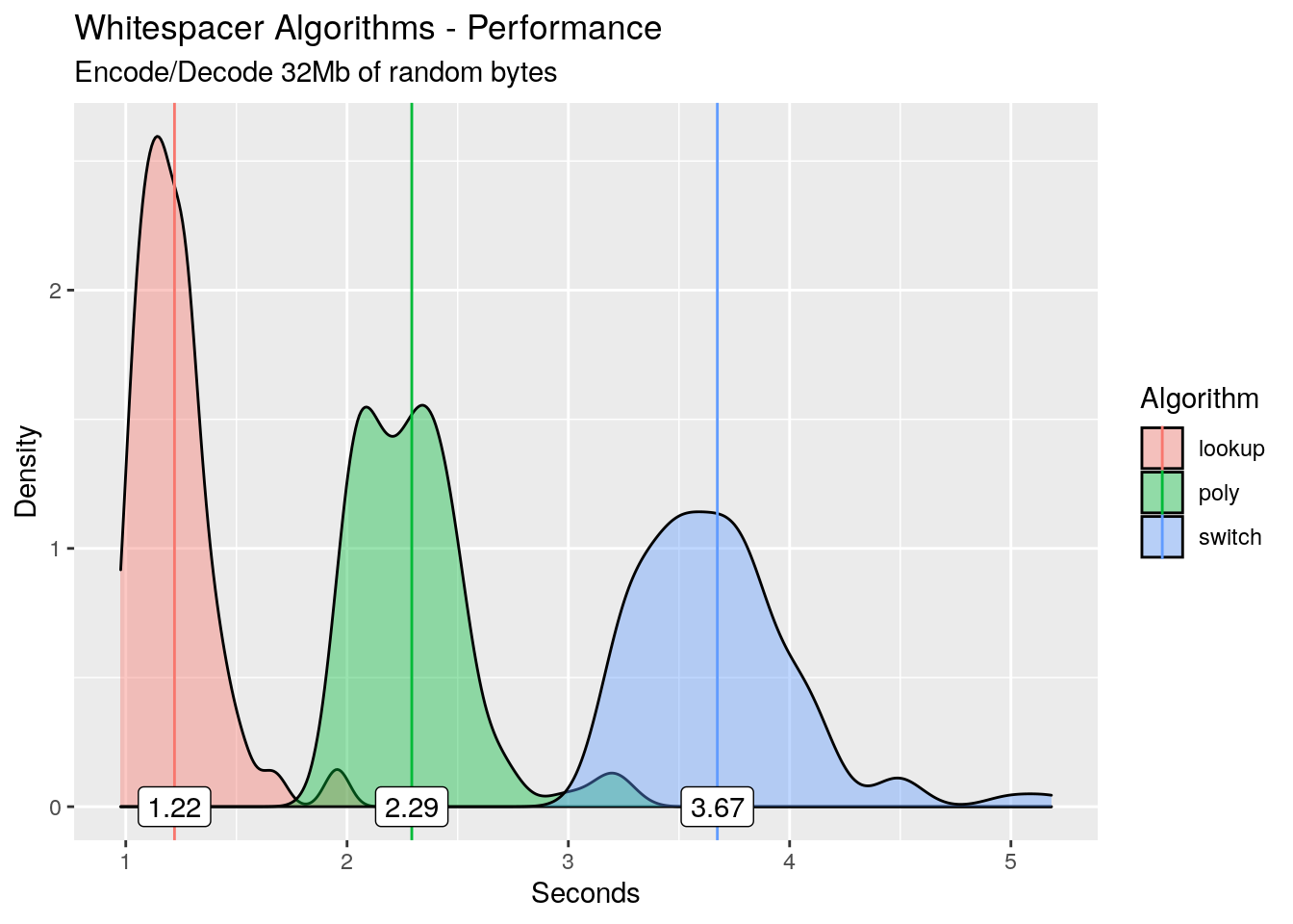
As expected, the polynomial encoding/decoding is slower than the lookup table. But what is really surprising is the switch statement: its slower than both! On average it’s 2.45 seconds slower than the lookup table! I love a good surprise, so let’s dive in and try to work out what’s happening.
What’s With The Switch?
We’ll take a bottom up approach and look at the instructions that were being executed on the CPU as the process was running. Using perf record we take samples of the process’s state, most importantly the instruction pointer. By using the -b switch, perf also captures the Last Branch Record (LBR) stack. With the LBR processor feature, the CPU logs the from and to addresses of predicted and mispredicted branches taken to a set of special purpose registers. With this information, perf can reconstitute the a history of the instructions executed, rather than only having a single point in time to use from the sample.
Let’s run the encoding half of the pipeline and feed it 32Mb of random bytes:
perf record -b -o switch.data -e cycles:pp ./ws_debug -a switch < urandom_32M > /dev/null
[ perf record: Woken up 22 times to write data ]
[ perf record: Captured and wrote 5.345 MB switch.data (6833 samples) ]
Looking at the trace data (saved in switch.data), the brstackins field allows us to see the instructions executed and approximate CPU cycles for different branches. Perf has captured around 43,000 executions of our switch_encode() function, with just one of these displayed below:
perf script -F +brstackinsn -i switch.data
switch_encode:
0000560dd2bffddd        insn: 55
0000560dd2bffdde        insn: 48 89 e5
0000560dd2bffde1        insn: 89 f8
0000560dd2bffde3        insn: 88 45 fc
0000560dd2bffde6        insn: 0f b6 45 fc
0000560dd2bffdea        insn: 83 f8 01
0000560dd2bffded        insn: 74 1e                     # MISPRED 4 cycles 1.50 IPC
0000560dd2bffe0d        insn: b8 0a 00 00 00
0000560dd2bffe12        insn: eb 0e                     # PRED 22 cycles 0.05 IPC
0000560dd2bffe22        insn: 5d
0000560dd2bffe23        insn: c3                        # PRED 5 cycles 0.20 IPC
Even without decoding the machine code, what immediately stands stand out is the 22 cycles taken following the branch misprediction. Let’s now zoom out and run perf stat to pull out some summary statistics:
# Perf stat with 32Mb urandom bytes
perf stat ./ws_debug -a switch < urandom_32M > /dev/null
 Performance counter stats for './ws_debug -a switch':

       1743.865268      task-clock (msec)         #    1.000 CPUs utilized
                 7      context-switches          #    0.004 K/sec
                 0      cpu-migrations            #    0.000 K/sec
            12,852      page-faults               #    0.007 M/sec
     6,484,859,596      cycles                    #    3.719 GHz
     5,773,682,725      instructions              #    0.89  insn per cycle
       967,903,800      branches                  #  555.034 M/sec
       123,207,223      branch-misses             #   12.73% of all branches

       1.744494500 seconds time elapsed
The first statistic that stands out are the instructions per cycle, which is just under one. The likely cause of this is the number is the number of branch misses, which is up at ~12%. These branch prediction misses are destroying any benefit of pipelining in the CPU.
I’ve got an sneaking suspicion that the cause of these missed branch predictions is our input data, so let’s test the hypothesis. We create a 32Mb file of all zeros from /dev/zero instead of random bytes, then re-profile with this data as input instead of the random bytes. I’ll omit the code and go straight to the results:
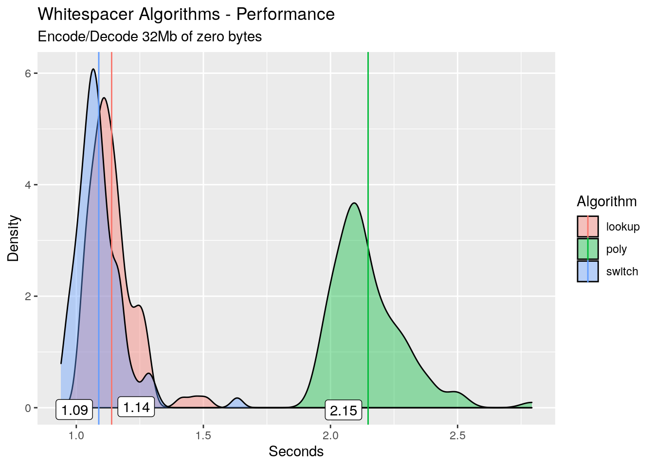
The switch algorithm now outperforms the others! Here’s the perf stat:
# Perf stat with 32Mb of zero bytes
perf stat ./ws_debug -a switch < zero_32M > /dev/null
 Performance counter stats for './ws_debug -a switch':

        543.503058      task-clock (msec)         #    0.999 CPUs utilized
                 8      context-switches          #    0.015 K/sec
                 0      cpu-migrations            #    0.000 K/sec
            12,854      page-faults               #    0.024 M/sec
     1,953,309,524      cycles                    #    3.594 GHz
     5,835,245,013      instructions              #    2.99  insn per cycle
       999,489,826      branches                  # 1838.977 M/sec
         1,226,487      branch-misses             #    0.12% of all branches

       0.544021460 seconds time elapsed
In the grand scheme of things, almost no branch prediction misses, and a huge speed increase as compared to the random bytes.
Now this is where I start to butt up against the limits of my CPU architecture knowledge (feel free to contact me with any corrections), but what I assume is happening is that the branch predictor on my CPU is using historical branching information to try and make good guesses. But when the input is random bytes, history provides no additional information, and the branch predictor adds no benefit. In fact it may be a hindrance due to the penalty of a missed branches.
Lookup versus Polynomial
Now let’s take a look at the unsurprising result: our original lookup algorithm versus the polynomial. We’ll go straight to using perf stat to see high-level statistics. First up is the lookup algorithm:
# Lookup table
perf stat ./ws_debug -a lookup < urandom_32M > /dev/null
 Performance counter stats for './ws_debug -a lookup':

        511.025199      task-clock (msec)         #    0.999 CPUs utilized
                 7      context-switches          #    0.014 K/sec
                 1      cpu-migrations            #    0.002 K/sec
            12,852      page-faults               #    0.025 M/sec
     1,802,617,592      cycles                    #    3.527 GHz
     5,195,307,808      instructions              #    2.88  insn per cycle
       487,513,834      branches                  #  953.992 M/sec
           506,448      branch-misses             #    0.10% of all branches

       0.511367875 seconds time elapsed
Now the polynomial:
# Polynomial
perf stat ./ws_debug -a poly < urandom_32M > /dev/null
 Performance counter stats for './ws_debug -a poly':

       1063.839451      task-clock (msec)         #    1.000 CPUs utilized
                 2      context-switches          #    0.002 K/sec
                 0      cpu-migrations            #    0.000 K/sec
            12,850      page-faults               #    0.012 M/sec
     3,829,284,007      cycles                    #    3.599 GHz
     7,755,413,038      instructions              #    2.03  insn per cycle
       487,472,058      branches                  #  458.220 M/sec
           537,512      branch-misses             #    0.11% of all branches

       1.064266885 seconds time elapsed
We see two main reasons as to why the polynomial is slower. First off it simply takes more instructions to calculate the polynomial as opposed to looking up the value in a lookup table. Second, even with the (likely cached) memory accesses, we’re able to execute more instructions per cycle with the lookup table as opposed to the polynomial algorithm.
Summary
In this article we looked at two different alternatives to a lookup table for encoding and decoding bytes in the whitespacer program. The fist was to try and use a polynomial function, and the second was to use a conditional switch statement.
We found a surprising result with the switch statement, and were able to determine using the perf tool that we were paying a penalty for missed branch predictions due to the randomness of the input data.
When you run into a problem or a surprising result, you’re often gifted an opportunity to learn something new. I’ve certainly learned a lot about perf, LBR stacks and branch prediction in putting this article together.