A Bit on the Nose
I’ve never been particularly interested in horse racing, but I married into a family that loves it. Each in-law has their own ideas and combinations of factors that lead them to bet on a particular horse. It could be it form, barrier position, track condition, trainer, jockey, and many others.
After being drawn into conversations about their preferred selection methods, I wanted come at the problem backed with data. I must admit I had an initial feeling of arrogance, thinking “of course I can do this better”. In fact I’ve seen this in many places where ‘data scientists’ stroll into fields of enquiry armed with data and a swag of models, but lacking an understanding of the problem space. Poor assumptions abound, and incorrect conclusions are almost certainly reached.
I was determined not to fall into the same traps, and after quashing my misplaced sense of superiority, I started to think about how to approach the problem at hand. Rather than diving straight into prediction - models akimbo - I thought the best place to start would be to create naive baselines. This would give me something to compare the performance of any subsequent models against.
In this article I will look at two baselines. The first is to pick a random horse in each race, which will provide us with a lower bound for model predictive accuracy. The second is to pick the favourite in each race. The favourite has many of the factors that we would be using in the model already built in via the consensus of the bettors: form, barrier position, trainer, jockey, etc. Any model we create needs to approach the accuracy of this method.
Simply put, we want to answer the following questions:
How accurate are our ‘random’ and ‘favourite’ methods at picking the winning horse?
What are our long term returns using the ‘random’ and ‘favourite’ methods?
Data Information & Aquisition
The data was acquired by using rvest to scrape a website that contained historical information on horse races. I was able to iterate across each race, pulling out specific variables using CSS selectors and XPaths. The dataset is for my own personal use, and I have encrypted the data that us used in this article.
The dataset contains information on around 180,000 horse races over the period from 2011 to 2020. It’s in a tidy format, with each row containing information on each horse in each race. It includes, but isn’t limited to, the name and state that the track, the date of the race, the name of the horse, jockey and trainer, the weight the horse is carrying, race length, duration, barrier position. Here’s an random sample from the dataset with some of the key variables selected:
hr_results %>%
    select(
        race_id, state, track,
        horse.name, jockey, odds.sp,
        position, barrier, weight
    ) %>%
    slice_sample(n = 10) %>%
    gt()
| race_id | state | track | horse.name | jockey | odds.sp | position | barrier | weight |
|---|---|---|---|---|---|---|---|---|
| 51226 | QLD | Doomben | Daisy Duke | Robbie Fradd | 6.00 | 1 | 3 | 58.0 |
| 134689 | VIC | Pakenham | Nautilus | James Winks | 6.00 | 4 | 1 | 54.5 |
| 24981 | WA | Bunbury | RABBIT NAGINA | Alan Kennedy | 31.00 | 6 | 10 | 56.5 |
| 78601 | NSW | Grenfell | Gaze Beyond | Ms Ashleigh Stanley | 6.00 | 4 | 9 | 53.0 |
| 44267 | NSW | Deniliquin | Sunpoint | Ms A Beer | 8.00 | 6 | 4 | 57.0 |
| 129895 | WA | Northam | Ram Jam | Ben Kennedy | 2.25 | 1 | 4 | 58.5 |
| 101574 | TAS | Launceston | Gee Gee Double Hot | Scarlet So | 5.00 | 1 | 1 | 52.0 |
| 134173 | VIC | Pakenham | Miss Mo | Ben E Thompson | 8.50 | 7 | 3 | 58.0 |
| 69517 | QLD | Gold Coast | Liberty Island | Jag Guthmann-Chester | 8.00 | 5 | 12 | 57.0 |
| 140862 | SA | Port Augusta | Gold Maestro | Jeffrey Maund | 31.00 | 1 | 5 | 54.0 |
We won’t use most of the variables in the data set, only a select few:
- race_id - a unique identifier for each race. There are multiple rows with the same race_id, each representing a horse that ran in that race.
- odds.sp - the ‘starting price’, which is are the “odds prevailing on a particular horse in the on-course fixed-odds betting market at the time a race begins.".
- position - the finishing position of the horse.
I’ve omitted the code to load the data, however the full source of this article (and the entire website) is available on github. The data is contained in the variable hr_results.
Exploration
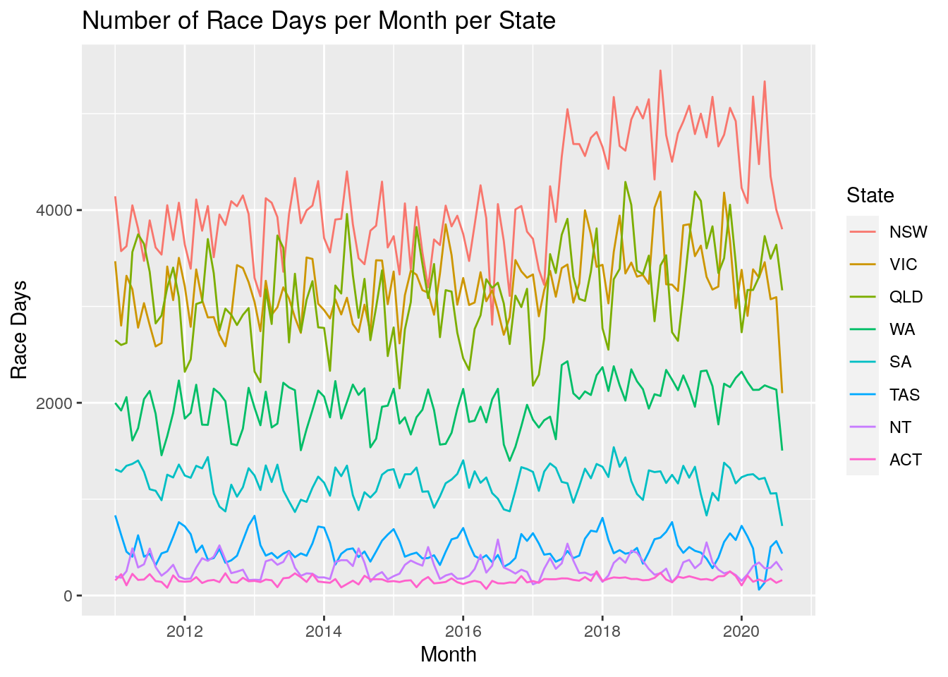
Let’s take a look at the dataset from a few different perspectives to give us some context. First up we take a look at the number of races per month per state. We can clearly see the yearly cyclic nature, with the rise into the spring racing carnivals and a drop off over winter.
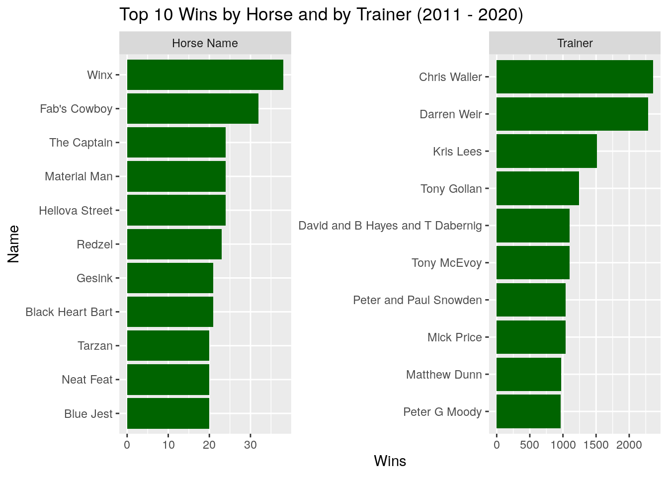
Next we take a look at the top 10 winning horses and trainers over this period:
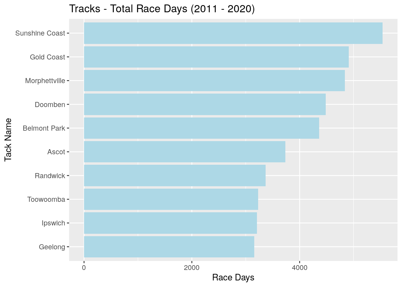
Which tracks have run the most races over this period?
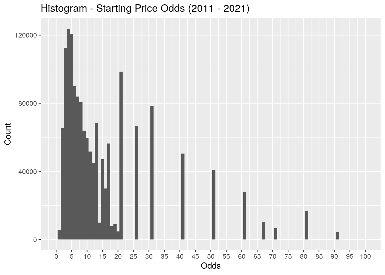
Finally, what is the distribution of the starting price odds? This distribution has a very long tail, so I’ve removed the long odds above 100 to provide a better view of the most common values. What’s interesting is the bias towards odds with round numbers after the 20 mark.
Data Sampling
With a high level handle on the data we’re working with, let’s move on to answering the questions. The process is:
- Take a sample of races across the time period.
- We will use 0.5% or ~800 races.
- Place a dollar ‘bet’ on a horse in each race, determined by one of our methods.
- Calculate our return (payout - stake).
- Calculate our cumulative return.
- Calculate our accuracy across all the races.
- Calculate our return per race.
- Return to 1. and repeat.
After the process is complete, we can look at the mean and distributions for the return per race and accuracy metrics. This process is similar to a bootstrap except within the sample we’re performing it without replacement instead of with replacement.
We select only the variables that we need, so we’re not moving huge amounts of unused data between to our worker processes. (Before I realised I should be pruning the data, I was spinning up large AWS instances with 128Gb of memory to perform the sampling. After the pruning I could run it on my laptop with 16GB of memory!) The data is nested based on its race ID, allowing us to sample per race rather than per horse.
# Nest per race
hr_results <- hr_results %>%
    select(race_id, position, odds.sp) %>%
    group_by(race_id) %>%
    nest()

head(hr_results)
## # A tibble: 6 x 2
## # Groups:   race_id [6]
##   race_id data
##     <dbl> <list>
## 1   25488 <tibble [6 × 2]>
## 2   25489 <tibble [5 × 2]>
## 3   25490 <tibble [6 × 2]>
## 4   25491 <tibble [12 × 2]>
## 5   25492 <tibble [14 × 2]>
## 6   25493 <tibble [9 × 2]>
The the mc_cv() (Monte-Carlo cross validation) function from the rsample package is used to create our sampled data sets. We’re not actually performing the cross-validation part, only using the training set that comes back from the function and throwing away the test set.
The worker function mc_sample() is created to be passed to future_map() so we can spread the sampling work across multiple cores.
We generate 2000 samples of .5% of the total races in the dataset, or around 800 races per sample. The returned results are unnested, returning us back to our original tidy format, with each sample identified by the sample_id variable:
# Sampling function that creates a Monte-Carlo CV set
# and returns the analysis portion.
mc_sample <- function(data, times, prop) {
    data %>%
        mc_cv(times = times, prop = prop) %>%
        mutate(analysis = map(splits, ~analysis(.x))) %>%
        select(-c(id, splits))
}

# Set up out workers
plan(multisession, workers = availableCores() - 1)

# Parallel sampling
number_samples <- 2000
hr_mccv <- future_map(
    1:number_samples,
    ~{ mc_sample(hr_results, times = 1, prop = .005) },
    .options = furrr_options(seed = TRUE)
)

# Switch plans to close workers and release memory
plan(sequential)

# Bind samples together and unnest
hr_mccv <- hr_mccv %>%
    bind_rows() %>%
    mutate(sample_id = 1:n()) %>%
    unnest(cols = analysis) %>%
    unnest(cols = data)
A bet_returns() function is created which places a bet (default $1) for the win on each horse in the dataset it’s provided. It determines the return based on the starting price odds. The data set uses decimal (also known as continental) odds, so if we placed a $1 bet on a horse with odds of 3.0 and the horse wins, our payout is $3, but our return is $2 (payout - $1). If the horse doesn’t win, our payout is $0 and our return is -$1.
# Places a bet for the win on each horse and calculates the return,
# the cumulative return, and the cumulative return per race.
bet_returns <- function(data, bet = 1) {
    data %>%
        mutate(
            bet_return = if_else(
                position == 1,
                (bet * odds.sp) - bet,
                -bet
            )
        ) %>%
        group_by(sample_id) %>%
        mutate(
            sample_race_index = 1:n(),
            cumulative_return = cumsum(bet_return),
            cumulative_rpr = cumulative_return / sample_race_index
        ) %>%
        ungroup()
}
Approach 1: Random Selection
The first approach to take is to bet on a random horse per race.
# Select a random horse from each race where there are odds available
hr_random <- hr_mccv %>%
    drop_na(odds.sp) %>%
    group_by(sample_id, race_id) %>%
    slice_sample(n = 1) %>%
    ungroup()

# Place our bets
hr_random <- bet_returns(hr_random)
Let’s first calculate the accuracy per sample, and view this as a histogram. The solid line is the mean, and the dashed lines are the 2.5% and 97.5% quantiles, showing the middle 95% range of the accuracy.
hr_random_accuracy <-
    hr_random %>%
    mutate(win = if_else(position == 1, 1, 0)) %>%
    group_by(sample_id) %>%
    summarise(accuracy = mean(win))
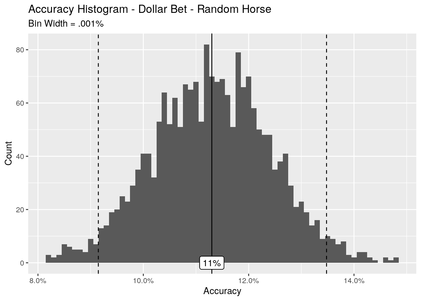
The random method gives us a mean accuracy of 11%, with 95% range between 9.1% and 13.5%. That’s about a 1 in 9 chance of picking the winning horse. At first I thought this was a little low, as the average number of horses in a race was about 6. I naively assumed that the random method would give us a 1 in 6 chance of picking the winnow, or 17% accuracy level. But this assumption assumes a uniform probability of winning for each horse, which of course is not correct.
Accuracy is one thing, but what about our returns? Let’s take a look at our cumulative returns over time. It’s difficult to graph the entire 2000 samples as it becomes one big blob on the graph, so we look at the first 40 samples which gives us a reasonable representation:
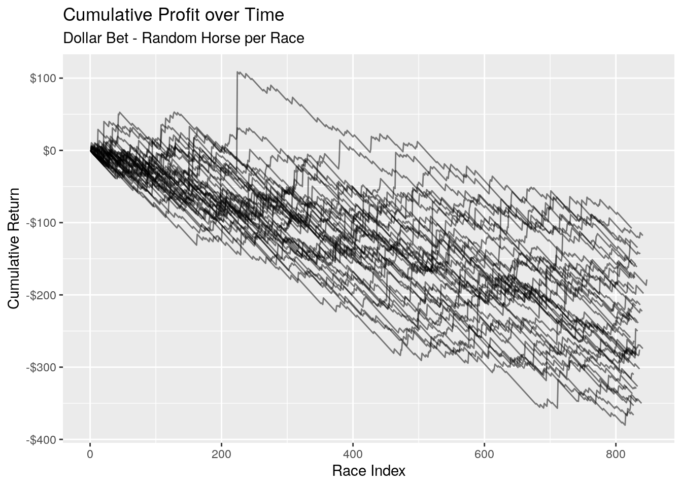
The result is a general trend downwards. We see some big jumps where our chosen horse is the long shot that came home, and some of our samples manage to pull themselves back into the black for periods of time. But they quickly regress trend back into the red.
The number of races may vary slightly per sample, so instead of looking at the cumulative return, let’s look at the returns per race, i.e. (cumulative return / number of races).
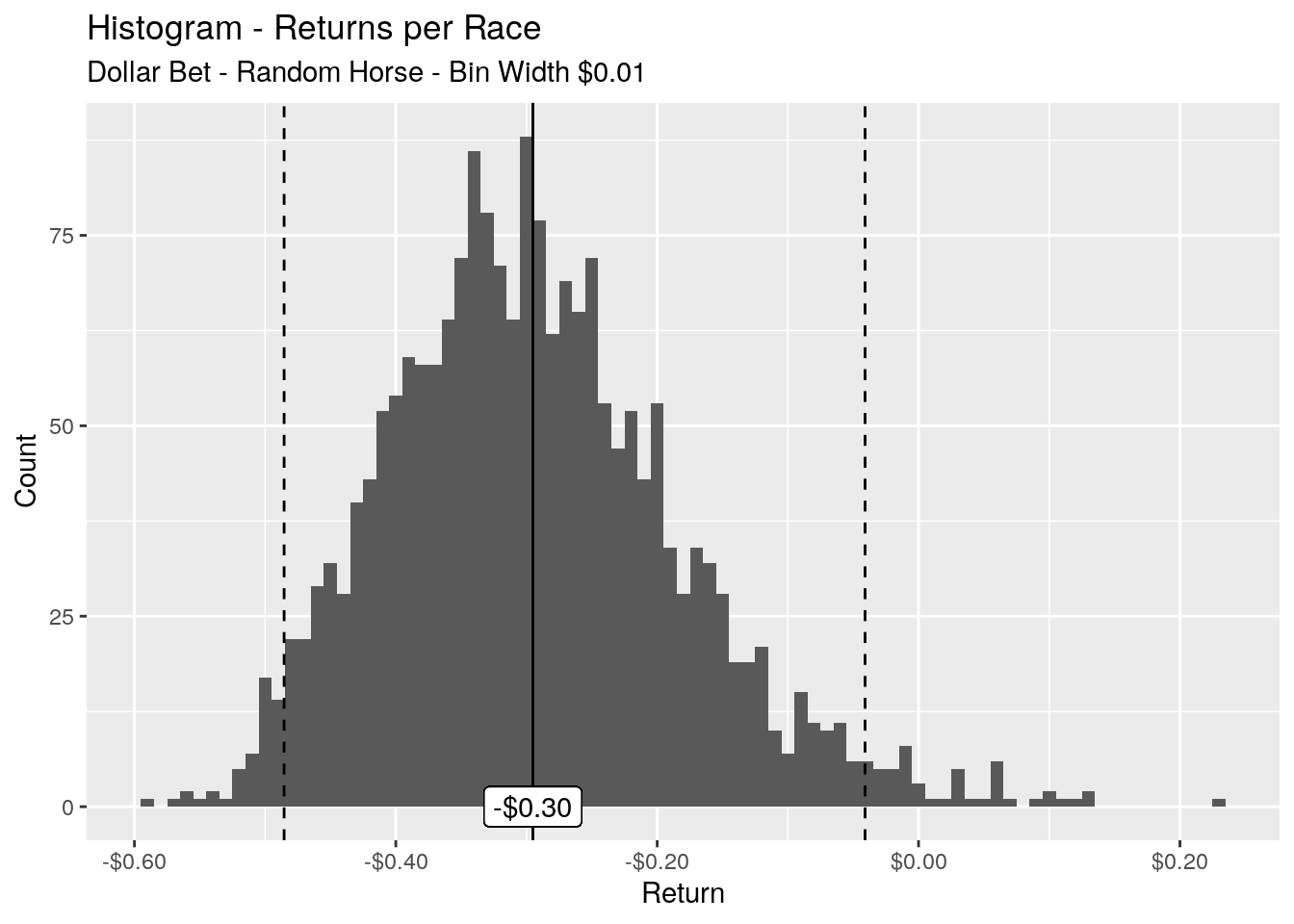
In the long run our average return per race is -$0.30, and 95% of our returns are within the range of -$0.49 to -$0.04. As we’ve used a dollar bet, this translates nicely to a percentage. What we can say is that in the long run we’re on average losing 30% of our stake each time we use this method of betting.
Approach 2 - Favourite
The second approach to take is to bet on the favourite in each race. We rank each horse in each race using the order() function, and extract the horse with a rank of 1. For races where there are two equal favourites, we pick one of those horses at random.
# Favourite horse from each race
hr_favourite <- hr_mccv %>%
    drop_na(odds.sp) %>%
    group_by(sample_id, race_id) %>%
    mutate(odds.rank = order(odds.sp)) %>%
    slice_min(odds.rank, with_ties = FALSE, n = 1) %>%
    ungroup()

# Place out bets
hr_favourite <- bet_returns(hr_favourite)
Let’s again take a look at the accuracy of this approach, viewed as a histogram of accuracy per sample.
# Calculate the accuracy
hr_favourite_accuracy <-
    hr_favourite %>%
    mutate(win = if_else(position == 1, 1, 0)) %>%
    group_by(sample_id) %>%
    summarise(accuracy = mean(win))
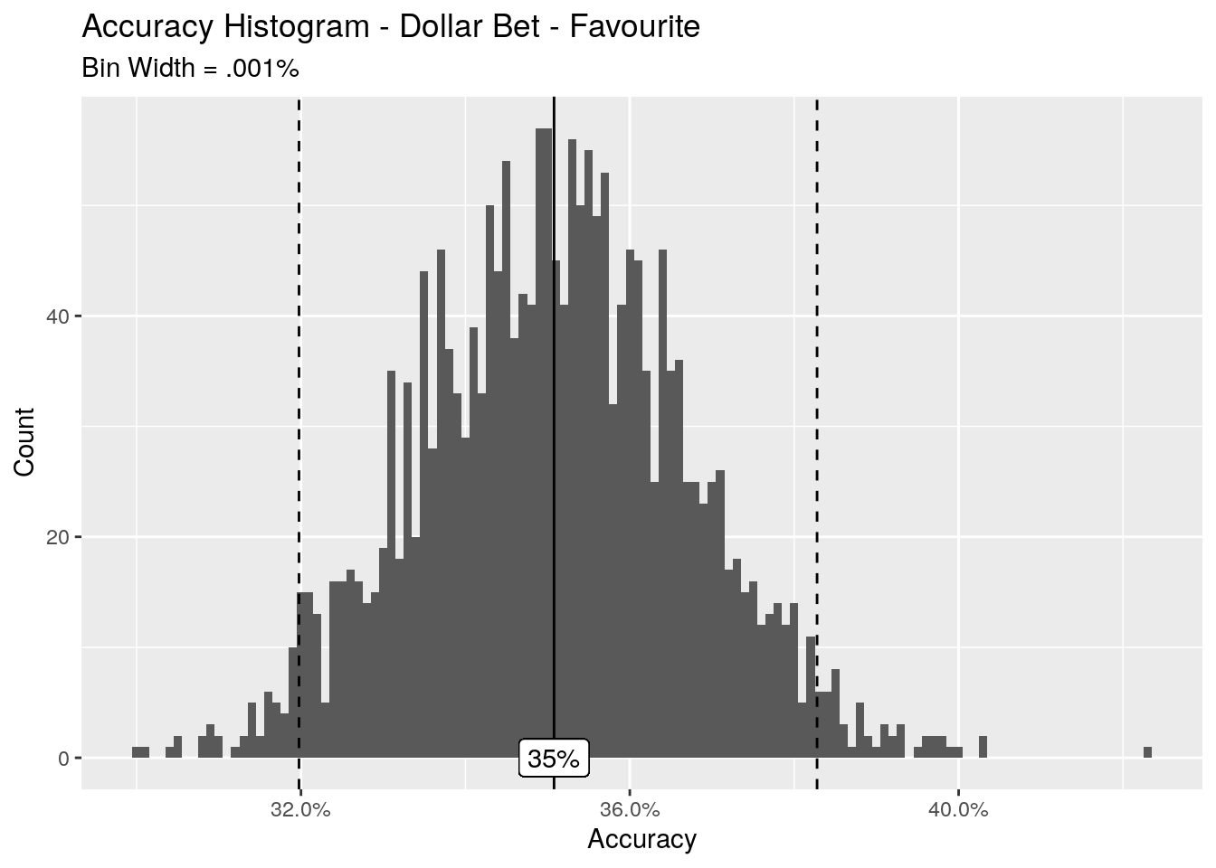
This is looking much better - we’ve got a mean accuracy across all of the samples of 35%, with 95% of our accuracy in the range of 32.0% - 38.3%. These accuracy percentages look pretty good, and my gut feel is that they would be pretty difficult to approach with any sort of predictive model. Picking the favourite is around 3 times better than picking a random horse.
What do our returns over time look like? Again we take the first 40 samples and graph the cumulative return.
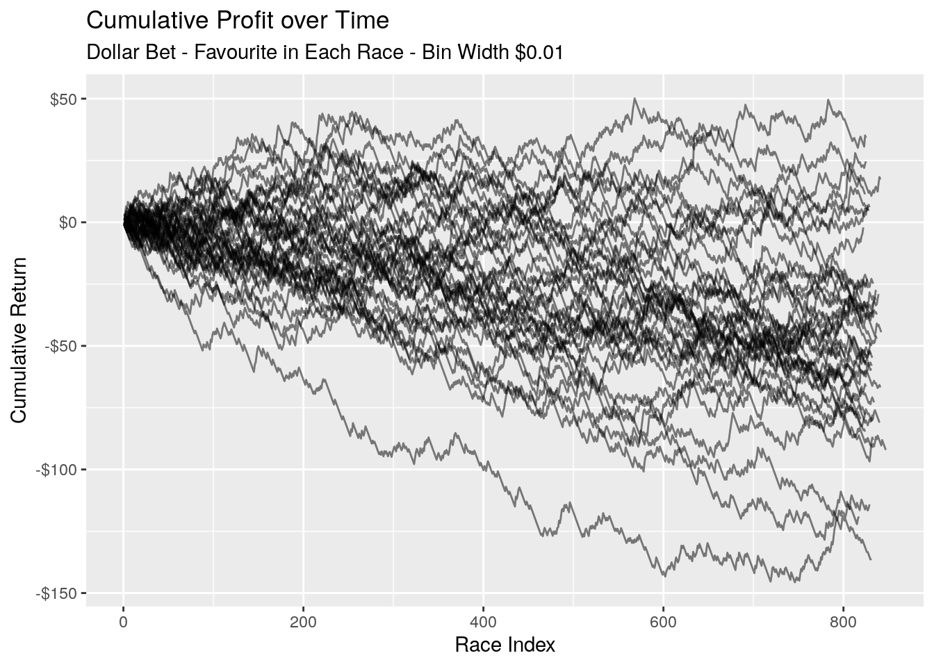
There is still a general trend downwards, however it’s certainly not as pronounced as the random method. There are longer periods of time where we’re trending sideways, and some of our samples even manage to eke out a profit.
Taking a look again at the distributions of our returns per race:
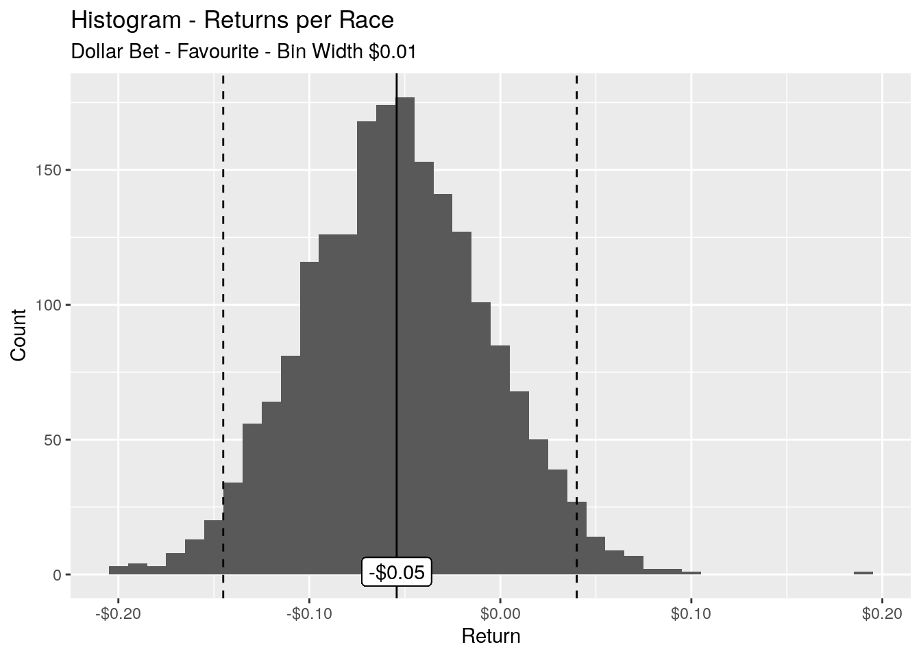
Picking the favourite is much better than picking a random horse but it’s certainly no slam dunk. The long run average return per race is still negative at -$0.05. The 95% of returns per race are in the range of -$0.15 to $0.04.
Conclusion
In this article we baselined two different approaches to betting on horse races: picking a random horse, and picking the favourite. Our aim was determine the mean accuracy and mean returns per race for each of the approaches.
We found the accuracy of picking a random horse is 11% and the mean returns per race for a dollar bet are -$0.30. You’re losing thirty cents on the dollar per bet.
Betting of the favourite is unsurprisingly much better, with a mean accuracy of 35% and mean returns per race for a dollar bet being -$0.05, or a loss a five cents on the dollar. I’m impressed with the bookies ability to get so close to parity.
What we don’t take into account here is the utility, or enjoyment, that is gained from the bet. If you think cost of the enjoyment you receive betting on a random horse is worth around 30% of your stake, or betting on the favourite is worth 5% of your stake, then go for it. As long as you’re not betting more than you can afford, then I say analyses be damned and simply enjoy the thrill of the punt.