Keeping Them Honest
Last month my car, a Toyota Kluger, was hit while parked in front of my house. Luckily no one was injured and while annoying, the person had insurance. The insurance company came back and determined that the car had been written off and I would be paid out the market value of the car. The question in my mind was ‘what is the market value?’ How could I keep the insurance company honest and make sure I wasn’t getting stiffed?
In this post I’ll go through an attempt to find out the market price for a Toyota Kluger. We’ll automate the retrieval of data and have a look at its features, create a Bayesian model, and see how this model performs in predicting the sale price of a Kluger.
More than anything, this was a chance to put into practice the Bayesian theory I’ve been learning in books like Statistical Rethinking and Bayes Rules! books. With any first dip of the toe, there could be assumptions I make that are incorrect, or things that are outright wrong. I’d appreciate feedback and corrections.
Finally, I won’t be showing as much of the code as I’ve done in previous posts. If you’d like to dive under the hood, you can find the source for this article here.
TL;DR
A word of warning before anyone gets too invested: this article is slightly anticlimactic. We do find that the sale price of a Kluger will reduce by around .6% for every 1,000 km driven, but there’s still a lot of variability that we dont capture, making our prediction intervals too wide to be of any use. There’s a other factors that go into determining a price that we need to take into account in our model.
But this isn’t the end, it’s just the start. Better to start off with a simple model, assess, and slowly increase the complexity, rather than throwing a whole bathtub of features at the model straight up. It also leaves me with material for another article!
Data Aquisition
The first step is to acquire some data on the current market for Toyota Klugers. A small distinction is that data will be the for sale price of the car, rather than the sold price, but it still should provide us with a good representation of the market.
We’ll pull the data from a site that advertises cars for sale. The site requires Javascript to render, so a simple HTTP GET of the site won’t work. Instead we need to render the page in a browser. We’ll use a docker instance of the webdriver Selenium, interfacing into this with the R package RSelenium to achieve this. This allows us to browse to the site from a ‘remotely controller’ browser, Javascript and all, and retrieve the information we need.
We connect to the docker instance, setting the page load strategy to eager. This will speed up the process as we won’t be waiting for stylesheets, images, etc to load.
rs <- remoteDriver(remoteServerAddr = '172.17.0.2', port = 4444L)
rs$extraCapabilities$pageLoadStrategy <- "eager"
rs$open()
Each page of Klugers for sale is determined by a query string offsetting into the list of Klugers in multiples of 12. We generate the offsets (12, 24, 36, …) and from this the full URI of each page. We then navigate to each page, read the source, and parse into a structured XML document.
kluger_source <-
    tibble(
        # Generate offsets
        offset = 12 * c(0:100),
        # Create URIs based on offsets
        uri = glue("{car_site_uri}/cars/used/toyota/kluger/?offset={offset}")
    ) |>
    mutate(
        # Naviate to each URI, read and parse the source
        source = map(uri, ~{
            rs$navigate(uri)
            rs$getPageSource() |> pluck(1) |> read_html()
        } )
    )
With the raw source in our hands, we can move on to extracting the pieces of data we need from each of them.
Data Extraction
Let’s define a small helper function xpt() to make things a little more concise.
# XPath helper function, xpt short for xpath_text
xpt <- function(html, xpath) {
    html_elements(html, xpath = xpath) |>
    html_text()
}
Each page has ‘cards’ which contain the details of each car. We ran into an issue is where not all of them have an odometer reading, which is the critical variable we’re going to use in our modelling later. To get around this, slightly more complicated XPath is required: we find each card by first finding all the odometer <li> tags, then using the ancestor:: axes we find the card <div> that it sits within. The result: we have all cards which have odometer readings.
From there, it’s trivial to extract specific properties from the car sale.
kluger_data <-
    kluger_source |>
    # Find the parent card <div> of all odometer <li> tags.
    mutate(
        cards = map(source,
            ~html_elements(.x,
                xpath = "//li[@data-type = 'Odometer']/ancestor::div[@class = 'card-body']"
            )
        )
    ) |>
    # Extract specific values from the card found above
    mutate(
        price = map(cards, ~xpt(.x, xpath = ".//a[@data-webm-clickvalue = 'sv-price']")),
        title = map(cards, ~xpt(.x, xpath = ".//a[@data-webm-clickvalue = 'sv-title']")),
        odometer = map(cards, ~xpt(.x, xpath = ".//li[@data-type = 'Odometer']")),
        body = map(cards, ~xpt(.x, xpath = ".//li[@data-type = 'Body Style']")),
        transmission = map(cards, ~xpt(.x, xpath = ".//li[@data-type = 'Transmission']")),
        engine = map(cards, ~xpt(.x, xpath = ".//li[@data-type = 'Engine']"))
    ) |>
    select(-c(source, cards, offset)) |>
    unnest(everything())
Here’s a sample our raw data:
Now some housekeeping: the price and odometer are strings with a dollar sign, so we need to convert these integers. We also create a new megametre variable (i.e. thousands of kilometers) which will the variable we use in our model. The year, model, and drivetrain are extracted out of the title of the advert using regex.
kluger_data <-
kluger_data |>
    mutate(
        odometer = parse_number(odometer),
        odometer_Mm = odometer / 1000,
        price = parse_number(price),
        year = as.integer( str_extract(title, "^(\\d{4})", group = TRUE) ),
        drivetrain = str_extract(title, "\\w+$"),
        model = str_extract(title, "Toyota Kluger ([-\\w]+)", group = TRUE)
    )
Taking a Quick Look
Let’s visualise key features of the data. The one I think will be most relevant is how the price is affected by the odometer reading.
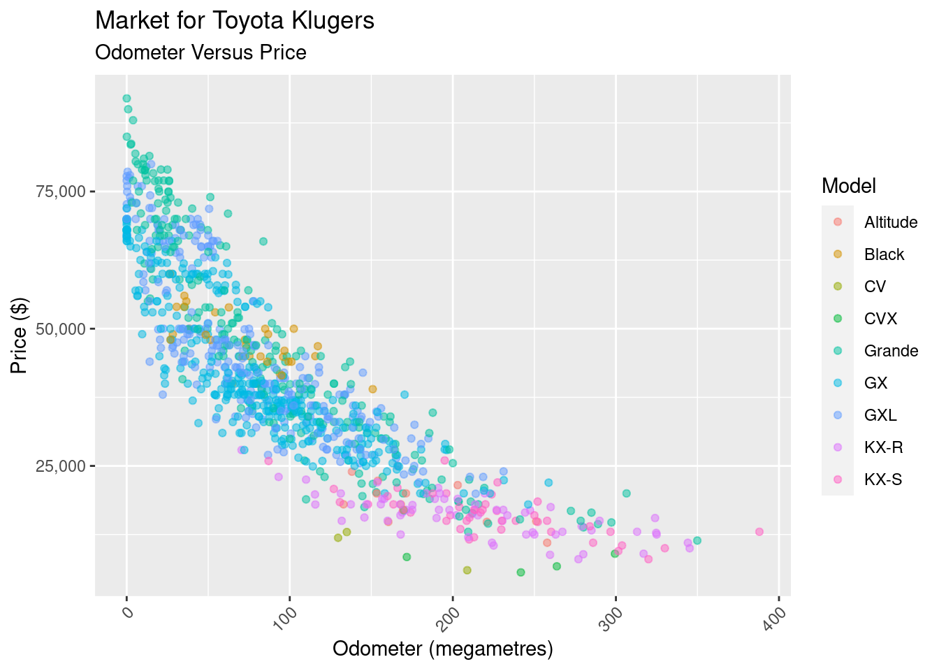 Nothing too surprising here, there more kilometers, the less the sell price. But what we notice is the shape: it looks suspiciously like there’s some sort of negative exponential relationship between the the odometer and price. What if, rather than looking odometer versus price, we look and odometer versus log(price):
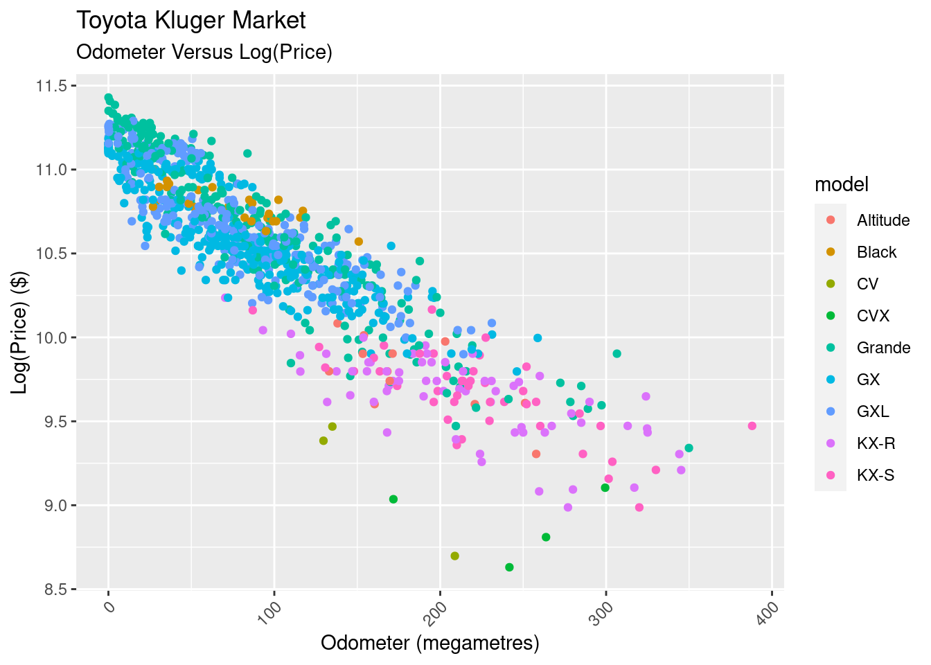 There’s some good news, and some bad news here. The good news is that the log transform has given us a linear relationship between the two variables, simplifying our modelling.
The bad news comes is that the data looks to be heteroskedastic, meaning its variance changes across the odometer ranges. This won’t affect our linear model’s parameters, but will affect our ability to use the model to predict the price. We’ll persevere nonetheless.
There’s nice interpretation of the linear model when using a log transformation. When you fit a line \(y = \alpha + \beta x\), the slope \(\beta\) is “the change in y given a change of one unit of the x”. But when you fit a line to to \(log(y) = \alpha + \beta x\), for small \(\beta\), \(e^\beta\) is ‘the percentage change in y for a one unit change of x’.
Where’s the the other variance coming from? Here’s the same view, but we split it out by model:
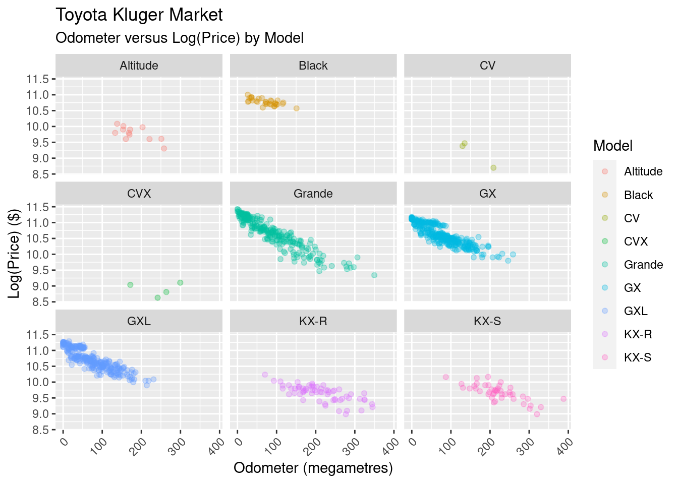
It barely needs to be stated, but the Kluger model has an impact on the sale price.
Modelling
Let’s start the modelling by thinking about the generative process for the price. Our observed variables odometer, year, model, and drivetrain are likely going to have an affect on price. There are some unobserved variables, such as the condition of the car its popularity that would also have an affect. There’s some confounds that may need to be dealt with as well: year directly affects price, but also goes through the odometer (older cards are more likely to have more kilometres). Model affects price, but also goes through the drivetrain (certain models have certain drivetrains).
The best way to visualise this is using the directed acyclic graph (DAG):
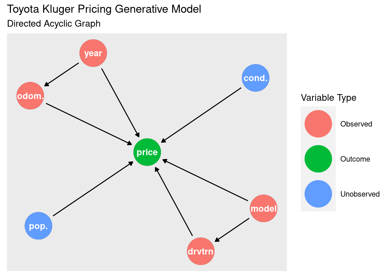
While I do have these variables available to me, I’d like to start with the most simple model I can: log of the price predicted by the odometer (in megametres). In doing this I’m leaving a lot of variability on the table, so the model’s ability to predict is likely going to be hampered. But better to start simple and build up.
At this point I could rip out a standard linear regression, but where’s the sport in that? Instead, I’ll use this as an opportunity to model this in a Bayesian manner.
Bayesian Modeling
I’m going to be using Stan to perform the modelling, executing it from R using the cmdstanr package. Here’s the Stan program:
data {
    int<lower=0> n;
    vector[n] odometer_Mm;
    vector[n] price;
}
parameters {
    real a;
    real b;
    real<lower=0> sigma;
}
model {
    log(price) ~ normal(a + b * odometer_Mm, sigma);
}
generated quantities {
    array[n] real y_s = normal_rng(a + b * odometer_Mm, sigma);

    real price_pred = exp( normal_rng(a + b * 60, sigma) );
}
It should be relatively easy to read: the data is our observed odometer (in megametres) and price, the parameters we’re looking to find are a (for alpha, the intercept), b (for beta, the slope), and sigma (our variance). Our likelihood is a linear regression with a mean basedon on a, b and the odometer, and a standard deviation of sigma.
There’s a conspicuous absence of priors for our parameters. If the priors are not specified, they’re improper priors, and will be considered flat \(Uniform(- \infty, +\infty)\), with the exception of sigma for which we have defined a lower bound of 0 in the data section. Flat priors aren’t ideal, as there is some prior information I think we can build into the model (\ \ is unlikely to be positive). But I’m going to do a bit of hand-waving and not put stake in the ground at this stage.
We’ll talk about the generated quantities a little later; these are used for validating the predictive capability of the model.
Let’s run the model with the data to get an estimate of our posterior distributions:
kluger_fit <- kluger_model$sample(
    data = compose_data(kluger_data),
    seed = 123,
    chains = 4,
    parallel_chains = 4,
    refresh = 500,
)
Running MCMC with 4 parallel chains...

Chain 1 Iteration:    1 / 2000 [  0%]  (Warmup)
Chain 2 Iteration:    1 / 2000 [  0%]  (Warmup)
Chain 3 Iteration:    1 / 2000 [  0%]  (Warmup)
Chain 4 Iteration:    1 / 2000 [  0%]  (Warmup)
Chain 2 Iteration:  500 / 2000 [ 25%]  (Warmup)
Chain 3 Iteration:  500 / 2000 [ 25%]  (Warmup)
Chain 1 Iteration:  500 / 2000 [ 25%]  (Warmup)
Chain 4 Iteration:  500 / 2000 [ 25%]  (Warmup)
Chain 2 Iteration: 1000 / 2000 [ 50%]  (Warmup)
Chain 2 Iteration: 1001 / 2000 [ 50%]  (Sampling)
Chain 3 Iteration: 1000 / 2000 [ 50%]  (Warmup)
Chain 3 Iteration: 1001 / 2000 [ 50%]  (Sampling)
Chain 4 Iteration: 1000 / 2000 [ 50%]  (Warmup)
Chain 1 Iteration: 1000 / 2000 [ 50%]  (Warmup)
Chain 1 Iteration: 1001 / 2000 [ 50%]  (Sampling)
Chain 4 Iteration: 1001 / 2000 [ 50%]  (Sampling)
Chain 2 Iteration: 1500 / 2000 [ 75%]  (Sampling)
Chain 3 Iteration: 1500 / 2000 [ 75%]  (Sampling)
Chain 4 Iteration: 1500 / 2000 [ 75%]  (Sampling)
Chain 1 Iteration: 1500 / 2000 [ 75%]  (Sampling)
Chain 2 Iteration: 2000 / 2000 [100%]  (Sampling)
Chain 2 finished in 3.9 seconds.
Chain 3 Iteration: 2000 / 2000 [100%]  (Sampling)
Chain 3 finished in 4.3 seconds.
Chain 4 Iteration: 2000 / 2000 [100%]  (Sampling)
Chain 4 finished in 4.9 seconds.
Chain 1 Iteration: 2000 / 2000 [100%]  (Sampling)
Chain 1 finished in 5.3 seconds.

All 4 chains finished successfully.
Mean chain execution time: 4.6 seconds.
Total execution time: 5.4 seconds.
Assessing the Model
What’s Stan done for us? It’s used Hamiltonian Monte Carlo to take samples from an estimate of our posterior distribution for each of our parameters a, b, and sigma. Now we take a (cursory) look at whether the sampling has converged, or whether some of the sampling has wandered off into a strange place.
The trace plot is the first diagnositc tool to pull out. We want these to look like “fuzzy caterpillars”, showing that each chain is exploring the distribution in a similar way, and isn’t wandering off on its own for too long.
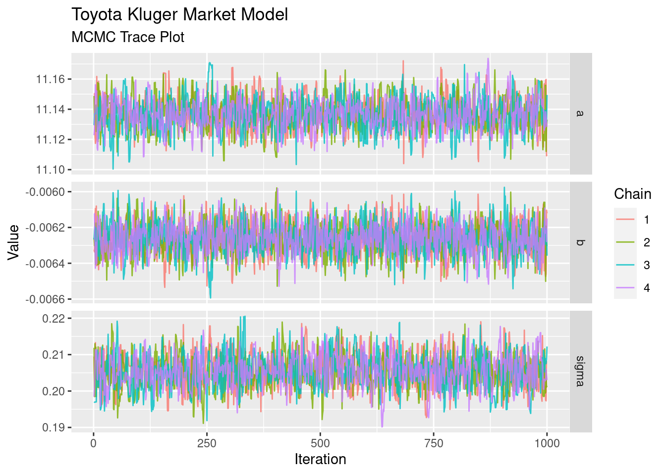 These look pretty good. That’s as much diagnostics as we’ll do for the sake of this article; for more serious tasks you’d likely look at additional convergence tests such as effective sample size and R-hat.
Taking the draws/samples from the posterior and plotting as a histogram we see the distribution of values that each of our four chains has come up with:
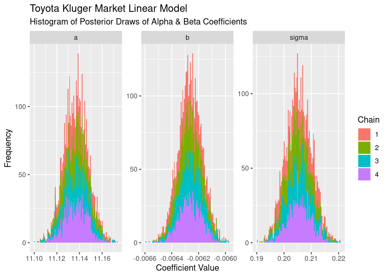 The first thing to notice it that, on the whole, each one looks Gaussian. Secondly, each of the chains has a similar shape, meaning they’ve all explored similar parts of the posterior. The intercept a has a mean approximately 11.13, and the slope b has a mean of approximately -0.0063. These are on a log scale, so exponentiating each of these values tells us that the average price with zero on tne odometer is ~$66k, and for every 1,000km the average price is ~99.3% what it was before the 1,000km were driven.
We’re not dealing with point estimates as we would with a linear regression, we’ve got an (estimate) of the posterior distribution. As such, so there’s no single line to plot. Sure we can take the mean, but we could also use the median or mode as well. To visualise the regression we take each of our draws and plot it as a line, effectively giving us the confidence intervals for the a and b parameters.
The confidence intervals are not very wide (which we saw in the histograms above). Looking at the 89% interval of the slope parameter we see it’s between -0.0061194 and -0.0064036. Exponentiating this and turning into percentages, we find that the plausible range for the decrease in price per 1,000km driver is between 0.610% and 0.638%.
The bad news is news we really already knew: the variance sigma around our line is large and it looks to be non-constant across the odometer values. A check to see how well this performed is posterior prediction, in which we bring sigma into the equation.
Recall the following line in our Stan program:
array[n] real y_s = normal_rng(a + b * odometer_Mm, sigma);
What we’re doing here is using the parameter posterior distributions, our model, and generating random draws to create a posterior predictive distribution for each odometer value. The idea is that, if our model is ‘good’, we should get values back that look like the data we’re modelling. In the plot below, I’ve filtered out values below 4.5% and below 94.5% to give an 89% prediction interval.
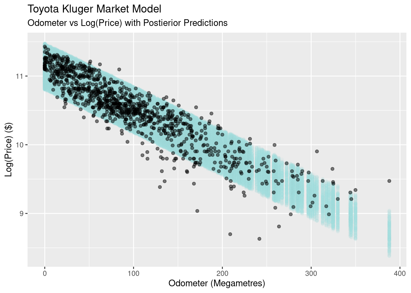 What we find is that the the predictive value of our simple linear model is not great. At odometer values close to zero it’s too conservative, with the all the prices falling well inside our predicted bands in light blue. At the other end of the scale the model is too confident, with many of the real observationsfalling outside of our predictive bands.
Another way to look at this is to look at the densities for both our model and the real values as the odometer values change. You can think of this as sitting on the above graph’s x-y plane, moving backwards along the odometer and looking at 10,000km slices of odometer values:
 This gives us a nice comparison of the models proablity density compared to the real data. At the start all of the data fits inside the 89% PI, and as we move along odometer values, the log(price) gets wider and falls outside outside of the modoels predicted area.
Despite these obvious flaws, let’s see how the model performs answering our original question: “what is the market sell price for a Toyota Kluger with 60,000kms on the odometer?” I’m using this line from the generated values section of the Stan model:
real price_pred = exp( normal_rng(a + b * 60, sigma) );
This uses parameters drawn from the posterior distribution, but fixes the odometer value at 60 megametres, and exponentiates to give us the price rather than log(price).
Here’s the resulting distribution of prices with an 89% confidence interval (5.5% and 94.5% quaniles):
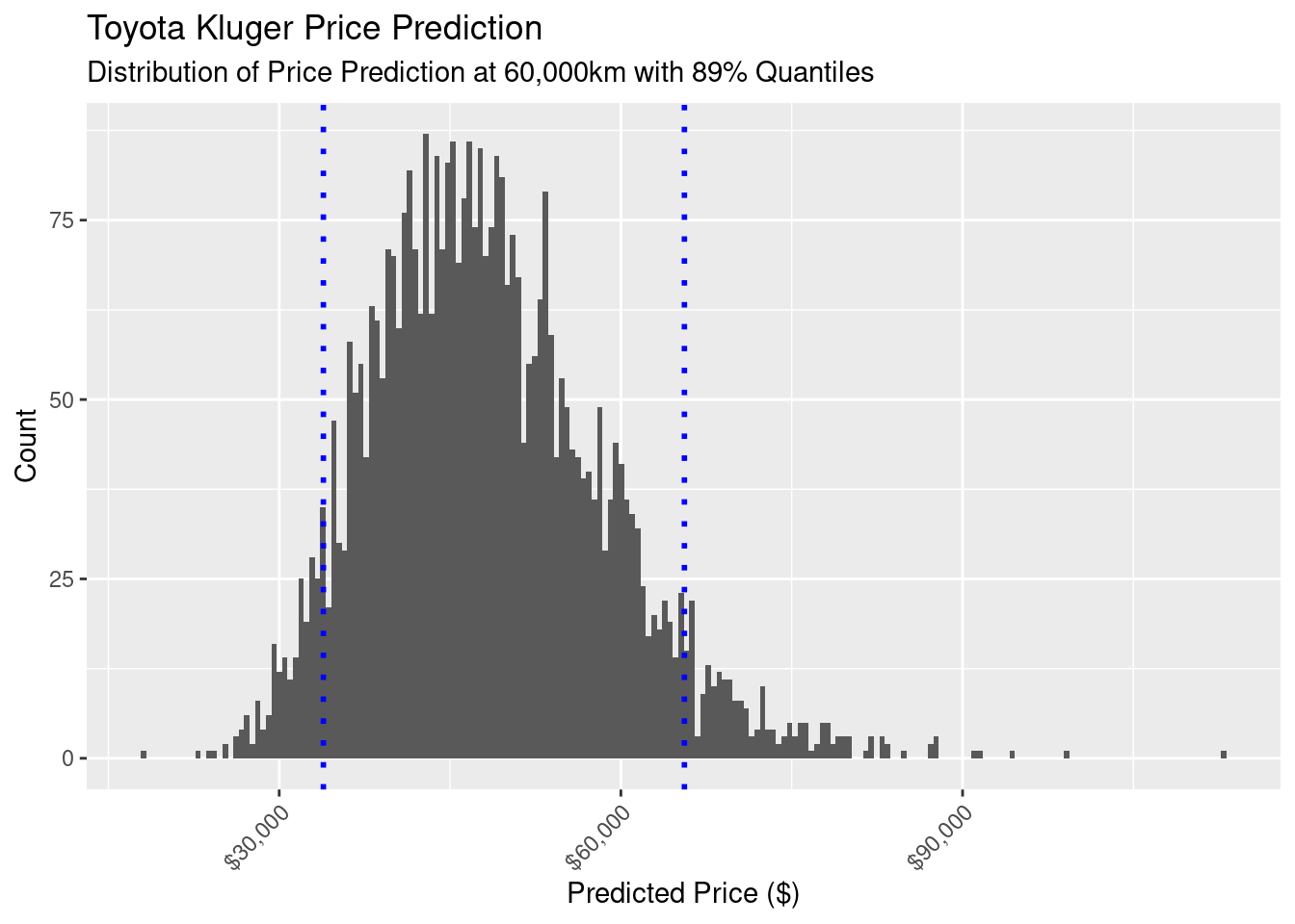 That’s a large spread, with an 89% interval between $33,878.97 and $65,575.44. That’s too large to be of any use to us in validating the market value the insurance company gave me for my car.
Summary
We’ve been on quite a journey in this article: from gathering and visualising data, to trying and validating new Bayesian modelling approach, to finally generating prediction intervals for the Kluger prices. All this, and at the end we’ve got nothing to show for it?
Well, not quite. Yes we’ve got a very simple model that doesn’t perform very well, but it is a foundation. From this, we can start to bring in other predictors that influence price. The next step might be to look at a hierarchical model that brings in the model of the Kluger. Maybe we can also find some data on the condition of the car? Sounds like a good idea for another post!